Assumptions of Disease Prediction Models

Introduction

Polygenic risk scores are a completely unknown, and therefore useless, quantity until they are properly evaluated. These evaluations are completed in the context of a model, for example a comparison of a polygenic risk score against a disease label can be considered an univariate linear regression. However, there are many factors that may confound a polygenic risk score, which is why most evaluations are multivariate models that contain common risk factors such as age and sex. Moreover, since disease is often considered an all or nothing affair we can use a logistic regression model, which better handles a binary covariate than a linear regression model. Now, most investigations of polygenic risk scores stop here and simply use a logistic regression model with a few basic covariates. However, just as logistic regression is better than linear regression, there are further model modifications we can make to produce a better model.

Although, it is important to note in this process that the descriptions of better, improved or enhanced are all difficult to objectively evaluate. Which is why we have to both consider the qualitative operation of the model modification and the quantitative effect on the prediction. While many, many model modifications are possible, we considered modifications that fall into five main catagories of assumptions. We will analyze these assumptions in turn:

Results

Representation of Age

First, in the vast majority of polygenic score models, age, which frequently influences disease risk, is only considered through the inclusion of a single covariate in a linear model. While the implied assumption that age has a linear relationship with disease risk is dubious in general, it is especially improbable in relation to polygenic risk scores, which are more accurate at predicting early onset, as compared to late onset, disease (see figure below). To better model the complexities of age two categories of variations are available. First, nonlinear age covariates, such as age squared, can be added to the model. Second, the cohort can be altered, for example the age distribution of individuals without disease can be made to match the age distribution of individuals with disease. Although, matched-cohort studies also carry a host of biases. Therefore, while age can certainly be better modeled in polygenic risk score analyses, and doing so may increase the effect of the scores, further investigations are needed to ensure all meaningful biases have been removed. While both categories of modeling variations are made in GWAS studies, they are rarely considered, to the best of our knowledge, within polygenic risk score analyses.

From these two general types of modified age representation models, I have implemented several variations to a plain model. The square and interaction models did this by adding either an age squared term, or an age squared and age to polygenic risk score interaction term to the set of plain covariates, respectively. The date of birth model variation exchanged the age at time of UK Biobank assessment with an age at the current date (relative to each individual’s date of birth), an age that is used by some investigations. The age stratified model variation split the training and testing phases into 5 year age groups, in which models were independently assessed. The prediction from each of these stratified models were averaged together to create results comparable to the other analyses. The narrow age model variation limited the training and testing phases to individuals aged between 56 and 64. Similarly, the age match cohort limited the training and testing phases such that the age distribution of the cases, or those with disease, and the age distribution of the controls, or those without disease, matched.

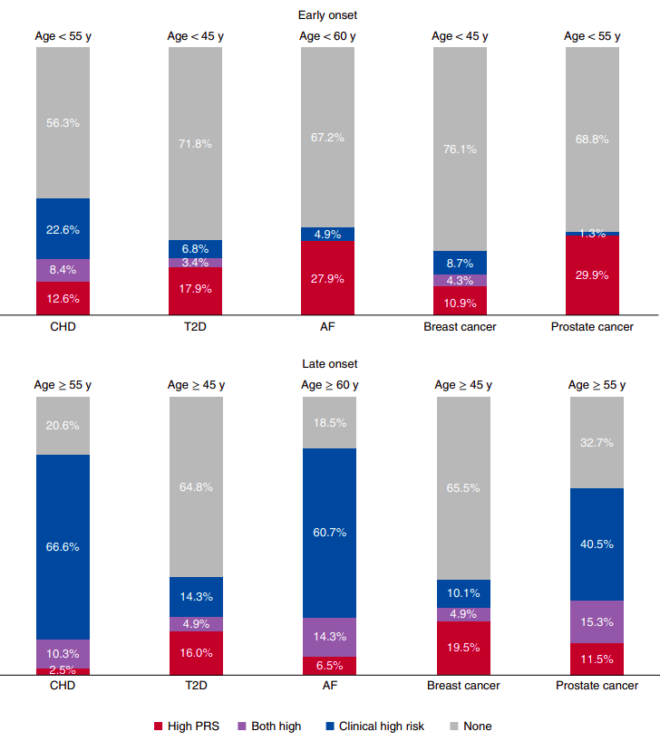
Figure 2 from “Polygenic and clinical risk scores and their impact on age at onset and prediction of cardiometabolic diseases and common cancers” by Mars. et al, published in Nature Medicine. The proportions of early- and late-onset cases with high clinical risk, high polygenic risk or neither. A high PRS is defined as one that is in the top decile of the distribution. The number of early- and late-onset cases for CHD was 190 and 1,019, for T2D 117 and 1,229, for AF 61 and 168, for breast cancer 46 and 696, and for prostate cancer 77 and 1,095. CHD, T2D and AF cases from FINRISK and breast and prostate cancer from FinnGen, all incident cases. The clinical high risk definitions were as follows: for CHD, the 10-year risk calculator for hard ASCVD ≥7.5%, according to the pooled cohort equations by ACC/AHA (2013); for T2D, a 10-year risk ≥33% when constructing a calculator with risk factors listed in the American Diabetes Association (ADA) criteria for testing for diabetes or prediabetes in asymptomatic adults; for AF, the 5-year risk of AF >5%, by a revised version of the CHARGE-AF; for breast and prostate cancer, a 10-year risk ≥5% with clinical risk factors.

Manner of Censorship

The time in which each individual survives without disease is quantified by the number of days since assessment. This approach creates an immortality bias within the individuals who were assessed at the end of the enrollment period, since they were unable to experience the disease during a period of time in which most other individuals in the study could. This participation bias is shared by several other high profile examples, such as a 1968 study of radiation exposure on Hiroshima atomic bomb victims. The bias can be reduced by recalculating each individual’s survival time in reference to a fixed date, forming a delayed entry model. Alternatively, each individual’s survival time can be calculated in reference to their date of birth. While models with delayed entry have been implemented in the wider epidemiological field, they have not to our knowledge been employed in conjunction with polygenic risk scores. And even as delayed-entry reduces this bias, it raises the question of time-scale. Several investigations reach conflicting conclusions on whether study-time or age-time is the preferred time-scale.

This topic can be very, very confusing as the vocabularly is not always clear, complex mathematical equations are often used to describe analytical frameworks, and the actual best method for analyzing the data is not clear. An excellent resource to cut through this confusion is “Survival Analysis: A Self-Learning Text” by Kleinbaum and Klein (which can be accessed here, particularly “Presentation X: Using Age as the Time Scale” starting on page 131. Much of the advice given within this book is drawn from the evidence presented in “Choice of time scale and its effect on significance of predictors in longitudinal studies” by Pencina et al. published in Statistical Medicine.

As I have alluded to in the previous paragraph, two delayed entry models were established to investigate the impact of censorship on the plain model. In addition, a model without censorship was used as a reverse type of comparison. The no censoring model variation changed the final end date of all individuals to the final date of the investigation, regardless of their event. The time variable was then calculated as the difference between the consistent, new end date and the date each individual was initially assessed. The delay entry by study time exchanged the typical right-censored survival object with a counting process survival object. For each individual, the first time in the counting process was calculated as the difference between their date of assessment and January 1st 2006, and the second time as the difference between their date lost to follow-up and January 1st 2006. The date January 1st 2006 was chosen as it occurred before any individual was assessed, and any change from this date did not model fitting. The term delayed entry is used because the model recognizes that the study starts on some actual absolute day and that the individuals were relatively delayed from one another in actually joining, and being observed in the study. The delay entry by age time changed the time basis from days in the study to days alive. Similar to the delay entry by study time model variation a counting process was employed. The first time was the difference between the date the individual was assessed by the UK Biobank and the individual’s date of birth, and the second time was the difference between the date the individual was lost to follow up and the date the individual’s date of birth. As age was implicitly counted by the model the explicit age term was dropped from the set of covariates. For both delay models a conversion from the delayed time frame to the plain model’s time frame was made such that the cumulative hazard values extracted from the delay analyses were measured at the same exact time, for each individual as was done originally for the plain model. Each of these analyses followed the same assessment procedure as the plain model.

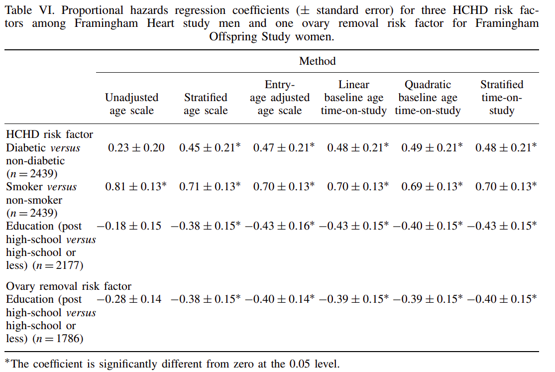Table extracted from Pencina et al.

Competing Risks

Standard cox proportional hazard models assume that all individuals will eventually be diagnosed with the disease, a poor approximation considering many individuals will die before the disease even begins to develop. The implementation of well-established competing risk models, such as multi-state or Fine and Gray, provide a ready correction to this assumption. Moreover, correcting for competing risks leads to absolute risk estimates, which are preferred within current real-world polygenic risk score implementations as they are easier to interpret in a clinical context. Despite the preference towards absolute risk estimates, the vast majority of models do not consider competing risks. Although, participation bias in the UK Biobank explicitly limits the time-extent of such predictions. Possible corrections to these biases, along with the use of improved multi-state schemes, may further exacerbate the accuracy differences between competing risk and plain models.

I considered competing risks, namely that of death, with several different model variations. The multi-state model considered competing risks by changing the binary phenotype variable to a categorical variable that includes the events of death, disease or censor. An important aspect of multi-state models is that they do not consider censoring to be informative, when they may in fact be because each individual entered the study at a different date and therefore likely a different age. The Fine and Gray model variation considers the event of death and changes the weight of each individual during cox proportional hazard model fitting. Unlike the multi-state model, the Fine and Gray model does not remove an individual from the risk pool when their competing risk occurs. While this appears unnatural, it better has been reported to better reflect the entire model whereas multi-state better reflects a specific individual. The multi-state model is directly available within the coxph function of the survival package, and the Fine and Gray model is available by using finegray function also from the survival package, then fitting a cox proportional hazards model with specified weights. The riskRegression model, from the riskRegression package, is highly similar to the multi-state model although it implements a different fitting algorithm.

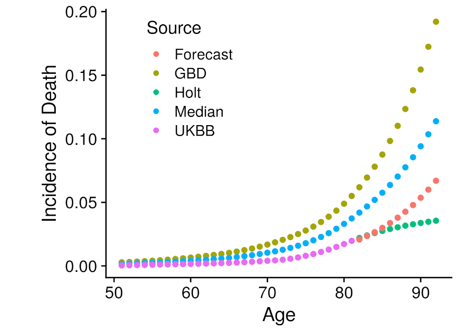
Another type of model required external data. Specifically that is the iCare models, from the iCare package, which implements a Gail style model that projects the risk estimated at one point in time into the future, incorporating all event incidence information. The advantage of this approach is that risk can be extended far beyond the currently known age-range of the cohort. Although, incidence information must be found from an external source. The external source we employed was the Global Burden of Disease Study, which had carefully constructed incidence estimates for most of the disease under analysis specific to the United Kingdom. Unfortunately, participation bias within the UK Biobank prevented us from directly utilizing the GBD information. To correct for the bias we developed several ways to combine the GBD data within empirically estimated UK Biobank disease incidence. The first left the GBD incidence values unchanged, the second extended the UK Biobank incidence values with the holt function, the third took the median between the GBD and Holt UK Biobank incidence values, and the fourth created a forecast model with the GBD values regressed against the UK Biobank values which then predicted the UK Biobank values beyond the available age. These four incidence estimates were all employed within an independent iCare model, creating four more analyses. Each of these analyses followed the same assessment procedure as the plain model.

Accuracy of Disease Labels

Disease labels, which determine the accuracy of risk predictions, are commonly based on unreliable sources. Electronic health records can be miscoded or partially unavailable due to a change in primary health provider, and self-reported records can be liable to an individual’s memory or perceptions. For example, 148 individuals with diabetes report HbA1c levels less than 35 mmol/mol, even though 48 mmol/mol is traditionally the diagnosis cut-off. The problem of unreliable disease labels is largely irremediable using current data collection mechanisms. However, patient data, such as HbA1c levels, blood pressure and BMI, can be used to predict a disease’s risk, such as Type II Diabetes. If a prediction derived from the patient data confidently disagrees with the disease label derived from electronic health records, then the corresponding suspect individual could be removed from the analysis.

Previous studies have demonstrated with evidence the accuracy of disease predictions derived from large datasets of patient data. For example, within the publication “Comparative analysis, applications, and interpretation of electronic health record-based stroke phenotyping methods” by Thangaraj et al. published in BioData Mining, a model developed with diverse features had an average AUC of 0.96 when predicting acute ischemic stroke. But to the best of our knowledge they have not assessed whether using disease predictions instead of direct disease labels effects the predictions of polygenic risk score models.

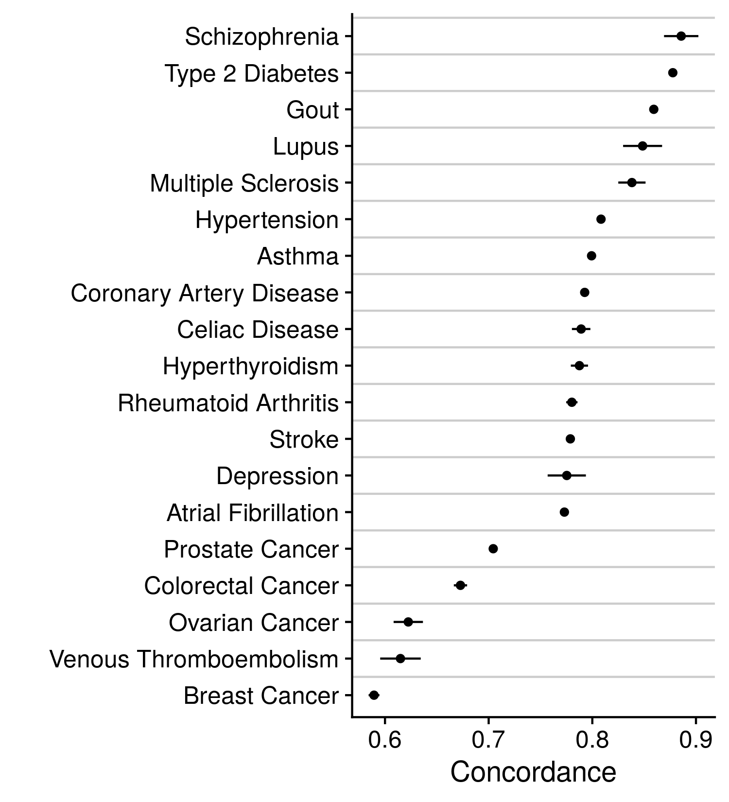
Our alternative approach to these disease labels was a model prediction that incorporated a wealth of information, such that one feature may be corrupted, and the larger prediction will remain relatively unchanged. Descriptions on how the disease prediction was made can be found earlier in this methods section. With the CoxNet model predictions we modified the current disease labels by either reclassifying individuals, changing their label to that identified by the prediction, or removing individuals, thereby reducing the size of the cohort. Either modification was only employed upon sections of the cohort that held very high or low disease predictions and did not or did previously report the disease, respectively. For example, individuals whose CoxNet model prediction was in the highest 5% amongst all individuals and were not positive for disease under the previous labels were removed or reclassified. Each of these analyses followed the same assessment procedure as the plain model. The accuracy of these models are indicated in the figure below.

Model Covariates

The features/covariates included in disease prediction models alongside the polygenic risk score are often manually and sparingly chosen. In this situation the polygenic risk score may become confounded, and thereby improperly represent an individual’s genetic risk. For example, a model of heart disease that includes the covariates of age, sex, BMI and family history may seem to contain all relevant features, yet blood pressure and/or smoking history may also be relevant to the prediction of heart disease. The application of a systematic feature selection process could unbiasedly determine which features should be included in a model so that the polygenic risk score is properly adjusted. While such processes do exist, to our knowledge nearly all investigations manually select a limited set of model covariates.

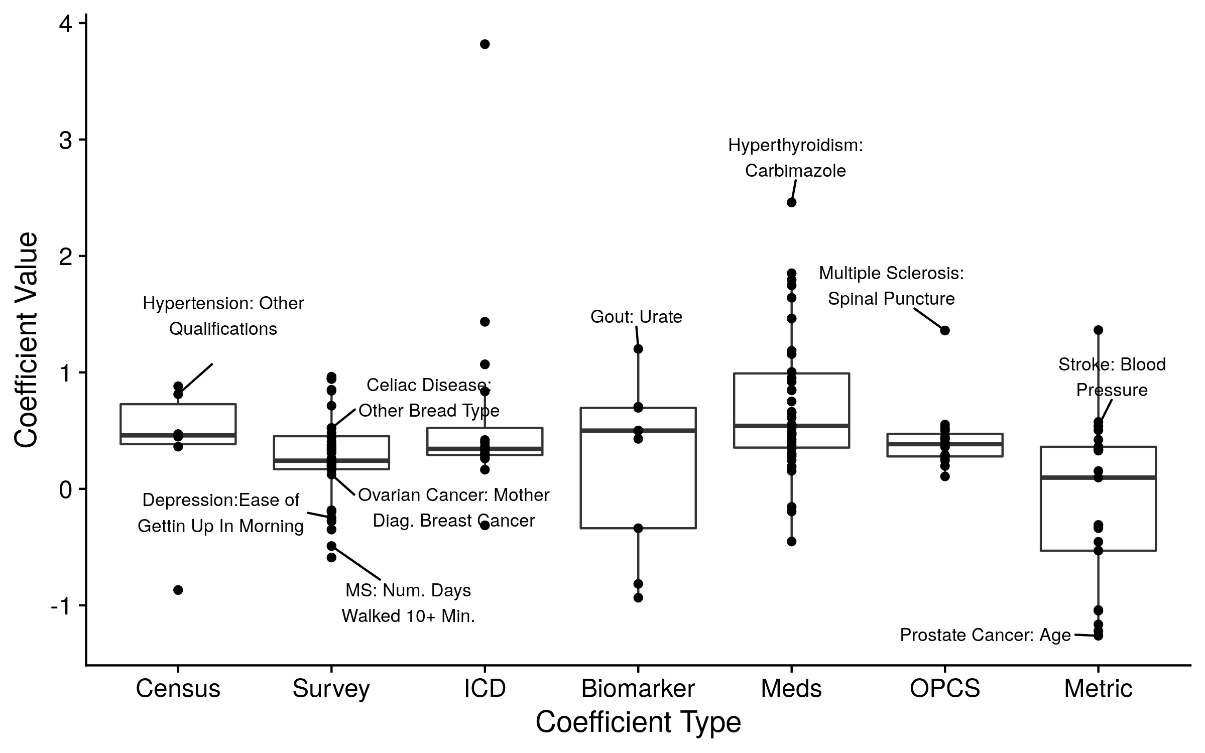
We therefore implemented an unbiased feature selection approach. Specifically, we used the covariates selected to be included in the CoxNet models described in the previous section. We either included all of the non-zero/included covariates, a group of the most important covariates (judged by the coefficient value), or the prediction from the CoxNet model. The top ten covariates from all of the models are displayed in the figure below. As expected, inclusion of additional covariates in the disease prediction model increased overall accuracy and decreased the value of the polygenic risk score. The polygenic risk score still contributed to nearly all disease prediction models. Although, our alternative predictions may be overfit or underperforming, leading to an underestimation or overestimation of each score’s effect, respectively. Further investigations are needed to determine proper, unbiased model adjustments.