Performance of Polygenic Risk Score Adjustment Methods
Introduction
A polygenic risk score is computed by multiplying the number of effect alleles by an externally determined effect size to form a single genetic variant prediction, then repeating the process and summing over all single predictions. This may sound complicated, but in essence it’s just the sum over many linear predictions, in which the prediction is calculated the same way any plain linear prediction is calculated. However, there are some very important considerations that are specific to this genomic situation.
First, the specific genetic variants that are included in the polygenic risk score. In theory, every single genetic variant (over ten million) could be included in the polygenic risk score sum. However, most of these millions of variants have no relation to the risk condition. Therefore, we want to select genetic variants that have some reasonably valid effect on the risk condition.
Second, the weights of the genetic variants that are included. The most likely true weight can be estimated through external linear regressions, or in other words an external genome wide association study.
However, a neat trick that many people like to pull is to include a genetic variant that has a questionable association to a disease but artifically decrease its effect size such that it has a very small impact on the overall polygenic risk score. Of course this neat trick is actually informed by very complex Bayesian algorithms.
When it comes to polygenic risk scores There are many other considerations or problems that many have worked on and generated solutions. These solutions can be though of as methods that take in a table of variants and effect sizes (often times the full summary statistics from a GWAS) and outputs a similar table of variants and effect sizes that can be used to construct the best performing polygenic risk score. Again, the ultimate objective of the methods is to generate a set of variants and effect sizes that can be used to calculate the maximally accurate polygenic risk score.
Available Methods
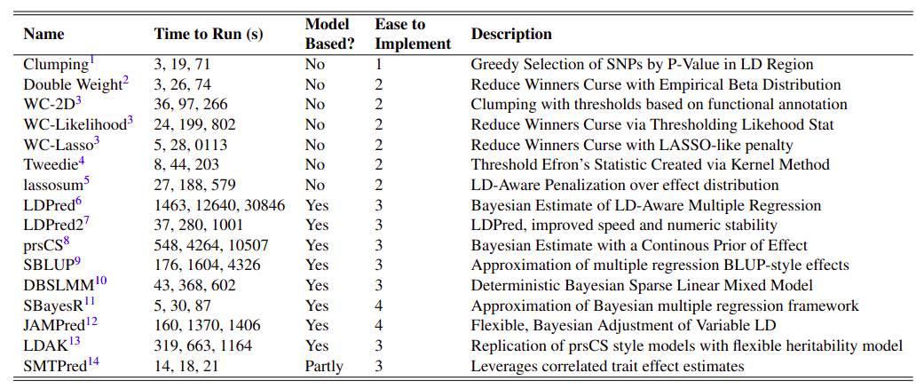
All of the methods that I will be discussing are listed in the following table.
Clumping
The clumping methods takes a very empirical, straightfoward approach to the problem of selecting variants that go into a polygenic risk score. After all, one of the more obvious and common approaches people take to selecting variants that relate to a phenotype is the application of a significance threshold, namely that the p-values is less than 5e-8. However, due to linkage disequilibrium several variants will all clump together, in one location or locus, each of which have very low, significant p-values. One of these variants is (likely) causing some biological event that leads to the phenotype whereas all of the other variants are just reflecting the allele identities of that likely causal variant. How do we identify the causal variant. Well that is a whole other area of study, but one of the fastest and simplest strategies is guessing that it is the variant with the lowest p-value amongst those in the locus. This is exactly what the clumping algorithm does, it goes to each locus selects the variant with the lowest p-value and pulls those into a table of variants that become the polygenic risk score.
Implementation of the clumping method was applied through the PLINK software. The “-—clump” flag was selected with a series of “-—clump-p1” p-value and “-—clump-p2” R2 thresholds, each of wich define exactly what an independent locus is. The variants in the output file were used to subset the primary summary statistics.
WC-2D
The clumping algorithm is simple, logical and effective - but there is room for improvement. For example, not all genetic variants are created equally. A genetic variant on a gene body is far more likely to cause some biological chage than a genetic variant in an intergenic region. Therefore, we might want to lower the signficance threshold of those variants in the gene body regions, as we have some other motivation for thinking the genetic variant is worthy to be included in a polygenic risk score. This idea of having two dimensions of threshold is implemented in the WC-2D method.
Implementation of the WC-2d (winners curse two dimensions) method roughly followed the steps outlined in the clumping method, except for specification of which regions clumping applies to. Specifically, variants identified as being conserved (listed within \url{http://compbio.mit.edu/human-constraint/data/gff/}) and pleiotropic (listed within supplementary table 2 of the respective publication) were both clumped with a higher p-value threshold. Only one of these varieties of variants were allowed to have a different threshold at a time.
WC-lasso
There is a concept called winner’s curse, which is best explained in terms of an auction. The person who has the highest bid wins the item for sale, but is cursed because they spent more money than anyone else wanted to. Similarly, a variant that is barely included or excluded in the final set of variants that forms a polygenic risk score is cursed. One way to avoid this curse is to minimize the effects of variants that are on the cusp of polygenic risk score inclusion. A popular way to determine which variants should be minimized, and exactly what that minimization should be is LASSO - a form of penalized regression. While LASSO is typically implemented in the context of a typical regression, a group of researchers have developed a mathematical workaround such that we can post-hoc complete LASSO. This workaround is called WC-lasso.
To implement WC-lasso (winners curse lasso), the original summary statistic file was first clumped with a p-value cut-off of 0.01 and R2 cut-off of 0.1. The vector of remaining effect sizes was then modified according to an equation that was extracted from the original publication.
The lambda value ranged from 0.001 to 0.1, and the output effect sizes were directly extracted without additional modification.
WC-likelihood
There is more than one way to try and eliminate winner’s curse. Another methedology looks to maximize the overall likelihood of the effects and p-values collected in variant set that is used to calculate the polygenic risk score. Specifically, as I understand it, this method assumes some underlying distribution of effect sizes then maximizes the selected effect sizes such that they fall under the high tail of this distribution. For lack of a better term this method is called WC-likelihood.
The WC-likelihood (winners curse likelihood) method was implemented similar to WC-lasso, with the same initial clumping step. The following effect adjustment step however required minimizing a likelihood function. The full function is available in the originating publication. Computationally, the minimization was accomplished by the Python function “minimize” and the “nelder-mead” method.
Double Weight
The Double Weight method, was implemented very similarly to the WC-likelihood and WC-lasso methods, even though it is not formally a member of the WC family. Specifically, the double weight method attempts to estimate the likelihood each variant belongs to a set of k top variants. The exact method it goes about calculating this probability of top variant inclusion is slightly complex, but it can be described as an inherently empirical process that looks at the similar variants to the one under analysis and makes an estimation. The surrounding process also follows the other WC methods.
After the initial clumping, the effects and standard errors were read into a custom written R script that simulated many samples of effects for each variant. Then a variant was selected to be in the final adjusted summary statistics if it was in the top range of SNPs with a specified probability. The value for the range of SNPs varied.
Originating Publication - Specifically, check the supplemental.
Tweedie
What I have called Tweedie’s method is highly similar to the WC-likelihood method. In fact, its motivation is identical. The only real difference is the form of the likelihood equation employed to estimate the true effect size of the genetic variants.
Implementation of the Tweedie method began by an application of the clumping method, following the steps as described in the original publication. For the initial clumping step the p-value threshold was set at 0.05 and R2 at 0.25. The modified summary statistic file was then used within the main tweedie R script that minimized a likelihood function similar to WC-likelihood. In order to extract the beta values the published script was modified slightly, and is located at https://github.com/kulmsc/PRS-Ithaca/blob/master/tweedy.R. Three variations of the betas were created, one for each of the FDR, Tweedie, and FDR x Tweedie sub-methods.
Originating Publication Official Documentation
LDpred
The LDpred method, in my reading of the literature, kick started the transformation from relatively simple, empirical clumping type methods to more advanced, modeling methods. The key model that LDpred is attempting to replicate is specifically a whole genome regression model. In other words, a typical GWAS will report summary statistics in which the effect of each variant is calculated independently. However, there are many other regression frameworks in which the effects of the variants are calculated all at the same time, which provides critical adjustments that limit the confounding caused by linkage disequilibrium. What LDpred does is convert the effect sizes from the independent linear regressions to effect sizes from the simultaneous, whole genome regression. Or at least, it tries to do this by taking advantage of an external linkage disequilibrium matrix. Within this process LDpred adds the further complexity of trying to estimate whether a variant has a true, causal effect on a phenotype. It completes this second task by considering some sub-distribution of variant effects, from the total distribution, that represent truly causal variants. The math gets a little complicated, and if you are interested you can check out another project I did which fully derives this LDpred method. But the key idea to understand, because it comes up again and again, is to combine LD patterns with simple, independent GWAS summary statistics to approximate complex, whole genome GWAS summary statistics through a bayesian framework.
To implement the LDpred method the starting summary statistic file was first converted into the STANDARD format required by LDpred (columns of chromosome, position, reference allele, alternative allele, reference allele frequency, info, rsID, p-value, and effect of the alterative allele). Generating this file simply required reorganizing the starting summary statistic file. The LD range was calculated as the number of SNPs divided by 4500. The “ldpred coord” step was first run, followed by a series of “ldpred gibbs” applications with various “f” values (the proportion of true causal variants).
Originating Publication Official Documentation
LDpred2
LDpred2 is theoretically identical to the original LDpred. The changes primarily involve computational re-workings of the bayesian algorithm that make it faster and easier to implement.
The implementation of LDpred2 directly followed the vignette that accompanied the original publication. While the theory was nearly identical to LDpred, all of the coding was done in R. Additional hyperparameters were fit to investigate a greater number of possible fractions of causal SNPs and heritabilities.
Originating Publication Official Documentation
lassosum
The lassosum method can be though of as a theoretical combination of both the WC-lasso and LDpred methods. LDpred because it understands that linkage disequilibrium is a problem that must be handled and that variants that likely do not have any true link to the disease should not be considered in a polygenic risk score calculation. WC-lasso because it decides that the best way to determine whether a variant does have a true link to the disease is not with multiple theoretical distributions of effect sizes, but rather the LASSO algorithm which shrinks the effects of variants that are deemed to likely not have any effect on the phenotype. This combination ends up with an algorithm that largely mirrors LDpred, except that the whole genome regression model that we are trying to replicate is now specifically a LASSO model.
Implementation of lassosum essentially required a single function call with UK Biobank used as reference data. The lassosum.pipeline function generated the adjusted effects with minimal intervention. A grid of “s” and “lambda” parameters were tried directly within this pipeline.
Originating Publication Official Documentation
PRScs
The PRScs methods is very, very similar to LDpred. The only difference is the way variants are judged to be truly causal or not. Specifically, LDpred uses what is called a point-slab prior in the bayesian process that approximates true causality. As the name states, PRScs instead uses a series of more flexible continous priors. This small mathematical change allows can potentially lead to a completely different selection of variants in the final set that are used to calculate a polygenic risk score.
Implementation of the PRScs first required converting the format of the summary statistics. The primary computation was encapsulated in the single python prscs call. The reference data employed was the European LD data listed within the PRScs documentation. The phi parameter was changed over three different function calls, whereas the a and b parameter were held steady.
Originating Publication Official Documentation
sBLUP
The sBLUP method is another variation on the LDpred theme of approximating the results of a whole genome style regression with only summary statistics from a GWAS in which variants were analyzed independently. What sBLUP does that is different, is specifically try to replicate a best linear unbiased prediction (BLUP) which is a certain random effect model. Therefore, we are again handling linkage disequilibrium, because of the whole genome replication, and are trying to again pick out the variants that likely have a true causal relationship to the phenotype by pulling apart the random and fixed effect of each variant. If you are confused about this last part do not worry, random effect models are rather complicated and are a little beyond the scope of this project, but if you are interested in learning more check out this guide, or look at others.
Implementation of the sBLUP method began by down sizing the original summary statistic to only the variants included within the HapMap (\url{https://www.broadinstitute.org/medical-and-population-genetics/hapmap-3}), and the columns were re-arranged to the MA format used throughout the GCTA tool kit. The actual sblup option was then run within gcta, with the wind option (the LD distance parameter) set to 100.
Originating Publication Official Documentation
SBayesR
The SBayesR is yet another variation of the LDpred theme (and sBLUP, and prsCS). SBayesR stands for summary bayesian alphabet, which suggests that this method attempts to replicate the results of a summary bayesian alphabet algorithm from the summary statistics of a GWAS which analyzed variants independently. The bayesian alphabet part of this description describes a complicated algorithm that found a key weakness in the BLUP, or generally fixed effect style of regression. Specifically, the fixed effect model assumes that all variants come from the same underlying distribution. In the simplest bayesian alphabet algorithm, each variant’s effect size is drawn from its own distribution with its own underlying variance. Other similar algorithms exist which make different assumptions, or priors, on this underlying distribution. For somewhat obvious reasons these bayesian whole genome regression algorithms can get exceedingly complex. For more information check out this review, or find another you prefer.
Implementation of the SBayesR method started similarly to sBLUP, with conversion of the summary statistics to the necessary MA format. The primary SBayesR computations were then run within the gctb toolkit. The ldm files were generated from the UK Biobank and down sized to HapMap variants, and could be downloaded directly from the documentation. Ldm files with more variants were not used due to size limitations.
Originating Publication Official Documentation
DBSLMM
DBSLMM stands for deterministic bayes spare linear mixed model, which is a mouthful. Once again, DBSLMM attempts to convert a set of GWAS summary statistics into an improved format that approximate a more sophisticated modeling framework. In this instance DBSLMM attempts to combine two of the previously discussed modeling frameworks, the random effects model of BLUP (hence the SLMM) and the abyesian alphabet of SBayesR (hence the B). The D, which stands for deterministic, is an added layer of algorithmic complexity that allows for a reasonably fast computational solution. Although, from experience, the many layers of modeling complexity make for a convergence problems.
Additional information was first derived, such as allele frequencies from a PLINK call applied to the UK Biobank data. Implementation of the DBSLMM algorithm was completed easily within a single R function call. Once generated p-value and R-squared hyperparameters were iterated over, and the adjusted effect sizes directly computed.
Originating Publication Official Documentation
SMTpred
SMTpred is a break from the strech of previously described model based methods. The key motivation behind SMTpred is that the genetic associations from one phenotype may help illuminate the genetic associations of another, similar phenotype. Genome wide association studies have utilized this idea within multi-trait BLUP models, which is similar to BLUP except that it harnesses the correlation between traits to better inform the underlying variation of the effect of the variants. From this model base, just like SBLUP, an algorithm is produced such that summary statistics from a simple GWAS can be adjusted to replicate the results of the multi-trait BLUP.
Implementation of SMTpred is unique in that it required not just the primary summary statistics being adjusted, but also summary statistics of similar diseases. The exact set of similar summary statistics are determined a priori through genetic correlation calculations. After proper formatting of the primary and similar summary statistics, they are all entered into a single python function call that adjusts the effect sizes. The number of similar sets of summary statistics varied. In addition, SBLUP adjusted effects are also utilized in this process.
Originating Publication Official Documentation
LDAK
Most of the methodology behind the LDAK adjustment is similar to that of PRScs, however the actual application has been custom-written and therefore requires far different inputs and operations. First, the summary statistics are converted into the proper format and a subset of the UKBB is converted such that the SNP identifiers are by position and allele, matching the style of externally downloaded annotation files. Next, per-SNP heritabilities are computed using the full BLD-LDAK heritability model, which includes 64 different types of annotations. The summary statistics are split three ways. In one split pseudo-summary statistics are computed, in another SNP-SNP correlations are computed. Next, the actual SNP adjustments are made assuming priors of lasso, lasso-sparse, ridge, bolt, bayes-r, and bayesr-shrink. For each model multiple parameters are tried, the best of which is determined via scoring with the third split of the summary statistics. High LD regions are removed if present, and the final adjusted effect sizes are substituted to form the final adjusted summary statistics.
Originating Publication Official Documentation
JAMPred
The JAMPred algorithm attempts to replicate a spare bayesian model, a somewhat similar idea as SBayesR.However, the exact details are different.
Implementation of the JAMPred algorithm is analogous to LDpred2 as both chiefly complete their computations within R. However, JAMPred is far less readily able to handle the large genotypic matrices necessary. Therefore, LD pruning in PLINK was first carried out, to reduce the size of the genotypic files. Next, the genotypic data is read into R using the bignsnpr package, and is then carefully converted into the necessary matrix specifications while still being in a memory-efficient format. The primary JAMPred function is then called over several iterations of lambda values, generating the adjusted effect sizes.
Originating Publication Official Documentation
Genetic Data
The aformentioned polygenic risk score methods were applied to data originating from the GWAS Catalog and UK Biobank. Specifically, the genotypic data from the UK Biobank supplied reference linkage disequilibrium matricies and the genetic information that eventually was utilized for scoring, and full summary statistics from the GWAS Catalog supplied a collection of genetic variants’ effect sizes.
Summary Statistics
Most summary statistics were acquired from the GWAS Catalog (https://www.ebi.ac.uk/gwas/downloads/summarystatistics). All studies were sought that had relatively high sample size, studied relatively prevalent, binary, disease traits, contained both minor and major alleles, and did not use UK Biobank data. In total 20 traits were chosen. All summary statistics were downloaded directly from the FTP server. Two additional summary statistics were acquired that were not within the GWAS Catalog. Migraine data from Gormley et al. came from a 23andMe data agreement, and anxiety and schizophrenia data came from the Psychiatric Genetic Consortium through their website (https://www.med.unc.edu/pgc/results-and-downloads). A brief description of each set of summary statistics utilized in this investigation is provided in table M4. A conversion script was deployed to regularize the various summary statistics. To only retain the highest quality single nucleotide polymorphisms (SNPs), a set of stringent criteria were assumed. If a SNP broke any of the rules in Table M5 it was removed from the larger summary statistics. In addition to the quality control, the alleles were either flipped or reversed to match the UK Biobank alleles by utilizing the snp_match function from the bigsnpr function. Lastly, the summary statistics were broken into a set for each chromosome.
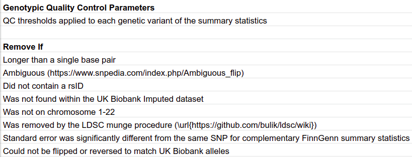
Table M5
UK Biobank
The UK Biobank is a very large, very well-informed data-set. Over 500,000 people were originally enrolled, all of whom were genreally between 40-70. These individuals were given an intensive questionaire, were genotyped with an array whose data was later imputed, were given blood/urine tests, and more. The specifics of the biobank is descibed in great detail in many other places, namely within the originating publication.
The UK Biobank imputed data was utilized to adjust summary statistics and create scores. Individuals not meeting the criteria listed in Table M1 were excluded. Processing of genetic material, except when required by specific adjustment methods, utilized the bgenix and PLINK utilities. The most efficient, and thereby utilized, combination of these utilities started with bgenix to subset the necessary SNPs, PLINK2 to complete additional QC, and PLINK1.9 to complete scoring, clumping or other computations. A final important note should be made that all of the genetic variants described are germline, held in common by nearly every cell in the body. While forms of cancer are discussed, somatic mutations are never utilized.
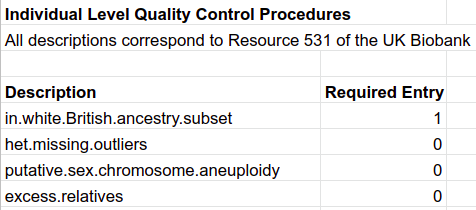
Table M1
Adjusting Summary Statistics
The summary statistics for each chromosome and GWAS were adjusted using various methods for the purpose of generating polygenic risk scores. The process of adjusting first requires the adjustment method, 16 of which were utilized in this investigation, all listed in the table at the top of the section. The various parameters that combined with each method to create the adjusted set of variants. Second, the set of summary statistics, listed in table M4 and previously quality controlled. Third, many methods require reference genetic data which often took the form of a small subset of UK Biobank data or alternative sources, namely the 1000 Genomes project. Fourth, a few methods required additional annotations. Each of these components were combined following the documentation described at the location the generative method was downloaded from. If any detail was missing in the documentation, then the accompanying publication was used. In this manner we did our best to apply each adjustment method exactly as the authors intended it. Although, we do understand that certain sets of summary statistics were sub-optimal, and the generative methods were not designed for their use. While the adjustment process varied in the actual adjustment computations, they all shared a beginning preparation step and a finishing step that substituted and/or subset the determined variant effects into the previous, original summary statistics.
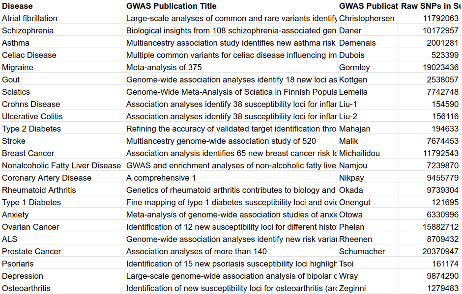
Table M4
As I have described so far there is a great deal of code that goes into this scoring process. While each of the methods have some form of publication and accompanying documentation, there is often times a very large gap between theoretical implementation and practical polygenic risk scores. For the full description of this process you will need to check out the full code repository, but for an example I will provide a snippet of the code used to execute the clumping method.
#The clumping file is submitted by a pipeline process
#The input variables therefore need to be set, as they are here
chr=$1
author=$2
dir=$3
low_author=`echo "$author" | tr '[:upper:]' '[:lower:]'`
d=comp_zone/dir${dir}


#There are multiple possible clumping parameters, for example the p-value and r2 thresholds
#the clump_param_specs file lists all of these parameters
#within this script I iterate over the different parameter options
i=1
cat all_specs/clump_param_specs | tail -n +2 | while read spec;do
  plim=`echo $spec | cut -f1 -d' '`
  r2lim=`echo $spec | cut -f2 -d' '`

  #want to double check that I have not already adjusted the summary statistics with
  # the current set of parameters
  if [ ! -e ~/athena/doc_score/mod_sets/${author}/${low_author}.${chr}.clump.${i}.ss ]; then

    #this is where the clumping actually happens, all with the PLINK tool
    #UK Biobank data is contained within the geno_files directly,
    # previously carefully extracted and processed for this purpose
    plink --memory 4000 --threads 1 --bfile geno_files/${low_author}.${chr}
       --clump temp_files/ss.${low_author}.${chr} --clump-snp-field RSID
       --clump-p1 $plim --clump-r2 $r2lim --out ${d}/out

    #If there were variants that were clumped, I want to extract those variant IDs and
    # use them to subset the entire gwas summary statistics
    if [ -f ${d}/out.clumped ]; then
      sed -e 's/ [ ]*/\t/g' ${d}/out.clumped | sed '/^\s*$/d' | cut -f4 | tail -n +2 > ${d}/done_rsids
      fgrep -w -f ${d}/done_rsids temp_files/ss.${low_author}.${chr} >
         ~/athena/doc_score/mod_sets/${author}/${low_author}.${chr}.clump.${i}.ss
    fi
  fi

  let i=i+1
done
Creating Polygenic Risk Scores
With the original GWAS summary statistics adjusted under various generative methods and respective hyperparameters, polygenic risk scores could be created. This computation was easily accomplished by using the “–score” option within PLINK1.9, and by following the genetic data processing workflow previously described. The “sum” option was included in the PLINK call to prevent normalization before the polygenic risk score for each chromosome was added together. To mitigate possible allele and variant mismatching, one genotypic file was created for each score that was needed. While this specificity slowed down the scoring, it appeared to reduce round-off error.
While there is less code required to calculate a polygenic risk score than adjust summary statistics, the code that is required is rather system specific and therefore not likely very helpful. However, I will display below the small snippet of code that actually extracts the necessary biobank data and then calls a PLINK command to calculate the polygenic risk score.
 #get the variants IDs that are within the score set of variants
 cat ../mod_sets/${author}/${ss_name} | cut -f3 > temp_files/rsids.${i}

  #pull out the score set of variants from the entire UK Biobank genotypes bgen file
  bgenix -g ~/athena/ukbiobank/imputed/ukbb.${chr}.bgen
     -incl-rsids temp_files/rsids.${i} > temp_files/temp.${i}.bgen

  #convert the bgen file into a PLINK (bed, bim, fam) file type
  plink2_new --memory 12000 --threads 12 --bgen temp_files/temp.${i}.bgen ref-first
     --sample ~/athena/ukbiobank/imputed/ukbb.${chr}.sample
     --keep-fam temp_files/brit_eid --make-bed --out temp_files/geno.${i}
  rm temp_files/temp.${i}.bgen

  #calculate the polygenic risk score
  plink --memory 12000 --threads 12 --bfile temp_files/geno.${i} --keep-allele-order
     --score ../mod_sets/${author}/${ss_name} 3 4 7 sum
     --out small_score_files/score.${low_author}.${chr}.${ver}.${method}

  #compress the polygenic risk score
  zstd --rm small_score_files/score.${low_author}.${chr}.${ver}.${method}.profile
As I mentioned, this is not the only way to calculate a polygenic risk score. Alternatively, you can calculate several polygenic risk scores from several sets of variants all at the same time. The variant set is just appended (column-wise) with other effect sizes that correspond to the other scores. This larger variant set can then be processed with PLINK2. While this system is much faster, in my experience the output does not perfectly align with the output of the above, split up style of code (although it is very close). So use at your own risk:
 #This is an R script that combines variant sets together into one large variant set
 #with multiple columns that correspond to multiple effect sizes
 Rscript align_sumstats.R $chr $cauthor

    #get all of the possible variant IDs required to compute the polygenic risk scores
    cat big_mod_set | cut -f1 | tail -n+2 > temp_files/all_rsid

    #figure out the number of polygenic risk scores to be calculated
    num_cols=`head -1 big_mod_set | cut -f3-300 | tr '\t' '\n' | wc -l`

    #extract the necessary variants from the entire UK Biobank dataset
    bgenix -g ~/athena/ukbiobank/imputed/ukbb.${chr}.bgen
       -incl-rsids temp_files/all_rsid > temp_files/temp.bgen

    #actually calculate the polygenic risk scores
    plink2_new --memory 12000 --threads 12 --bgen temp_files/temp.bgen ref-first
       --sample ~/athena/ukbiobank/imputed/ukbb.${chr}.sample --keep-fam temp_files/brit_eid
       --score big_mod_set 1 2 header-read cols=+scoresums --score-col-nums 3-${num_cols}
       --out big_small_scores/res.${chr}.${low_author}

    rm temp_files/temp.bgen temp_files/all_rsid big_mod_set

    #compress the resulting scores
    gzip big_small_scores/res.${chr}.${low_author}.sscore
Tuning to the Best Score (For Each Disease)
The best generative method and set of respective hyperparameters for each disease was determined through application of cross-validation within a training phase of the UK Biobank. Specifically, the tuning process began with only 60% of all British individuals who passed QC. Then three folds were iterated through in which two thirds of the data was used for training and the remaining third for testing. These folds were themselves repeated three times, shifting the start of the index that determined the three groups by one ninth of the total population. This method is commonly called repeated cross fold validation.
Within each fold of the cross-validation a logistic regression model was fit to the training data. This model regressed the covariates of age at time of assessment, sex, top ten genetic principal components and a polygenic risk score against the binary disease labels. The model’s predictions of the testing data were compared to the actual disease labels of the testing data, generating a receiver operator curve, from which the area under the curve, or AUC was computed. Once all folds were complete the AUC values were averaged over the nine folds. From these averaged AUCs the greatest value corresponds to the best polygenic risk score.
Unfortunately, there is a tremendous amont of code that goes into creating this cross validation framework, setting up the proper data frames, and then forming the models and statistics. There is not even a particularly good snippet to show. So please, check out the full code repository if you are interested. The accuracy results, stratified according to method, looks as follows:
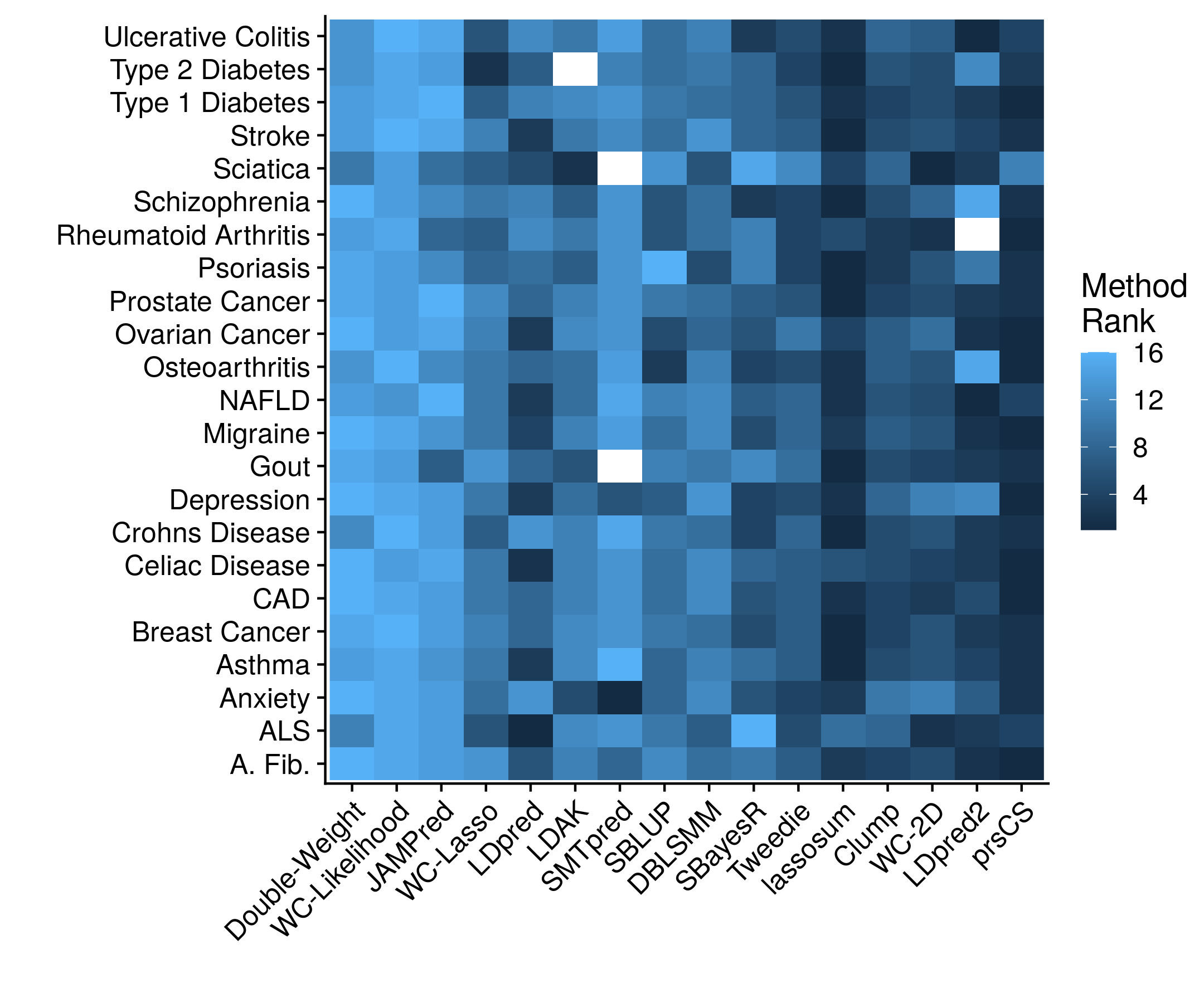
Now stratifying across all of the diseases prevents a clear determination on which method is actually working the best. Which is why we can collapse the disease dimension by simply taking the mean rank.
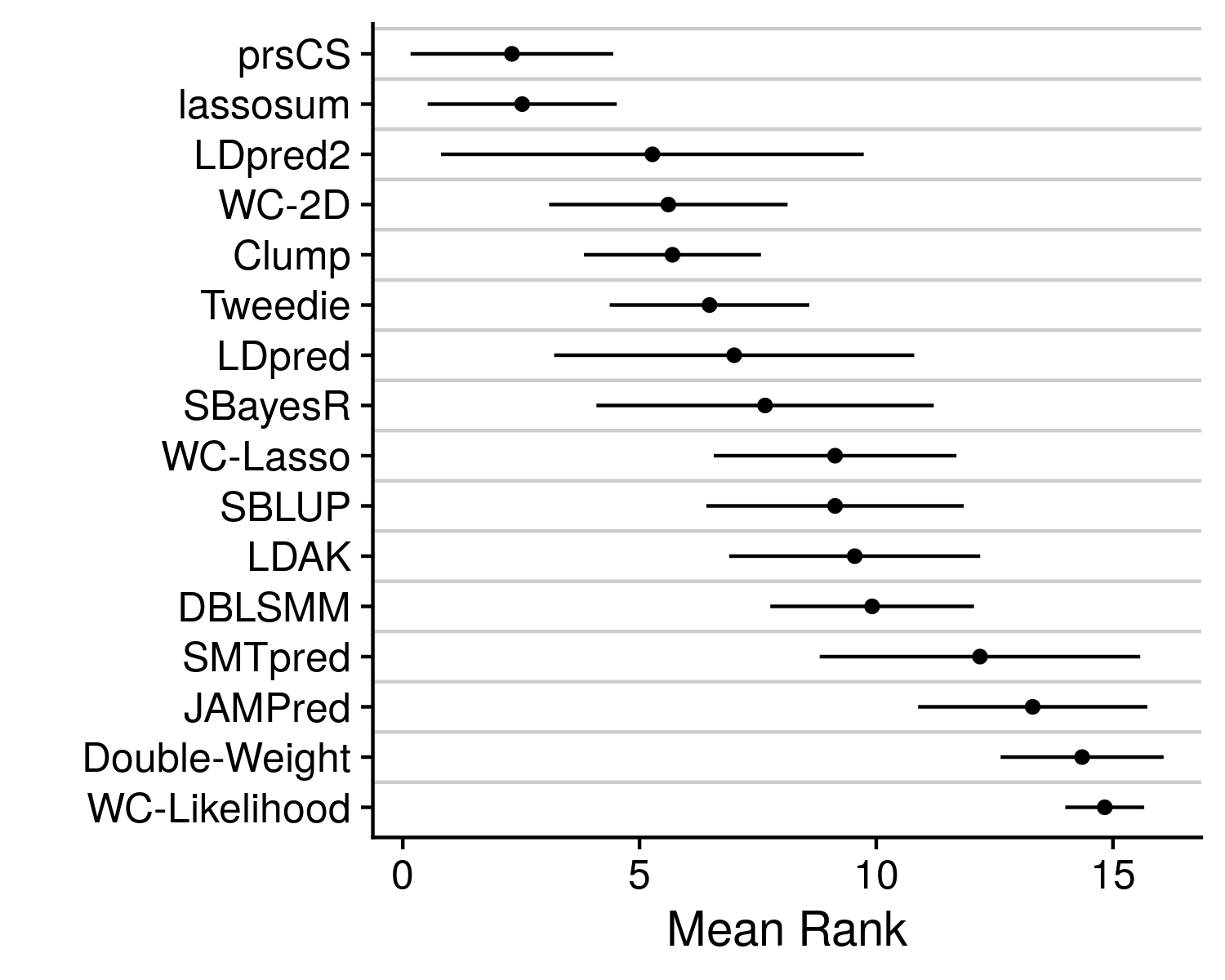
We see that prsCS, lassosum and LDpred2 are all the preferred methods. Although, there is a good deal of variance in this mean rank statistic. To get a final improved understanding of which method is the best we can go back to the originating accuracy statistic, AUC.
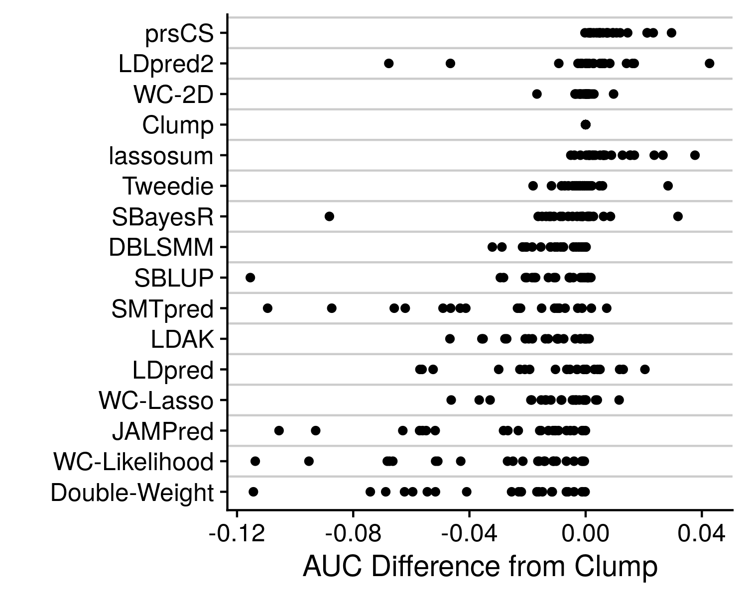
Rather than just displaying the AUC, I take the difference from the clumping AUC, which being the simplest method provides a nice baseline to compare to. We can see that some other methods, such as SBayesR and Tweedie, can also occasionaly produce high accuracy values, and should therefore likely not be discounted as poor methods. And again we can see great variance in performance, that is largely dependent on the genetic architechture of the disease under analysis. However, the simple and easiest take away here is that prsCS is the single, best method to employ, although in general any well thought out AND easy to implement model-based polygenic risk score method will produce an impressive polygenic risk score that will likely serve your needs perfectly well.