10 Additional Testing Statistics
Soon after carrying out the framework for polygenic risk score analyses reported in the previous section I realized that far more statistics exist that can be computed. Even better, these statistics are often far more interpretable by a clinical audience, the audience that matters. I therefore set about writing code that simply computed all of these additional statistics and later on plotting them in a clear way. I will pull out the relavent code for each statistic and describe why it is being computed. At the end I will include the full code (each of the statistical computations are intertwined into the base and score and extra covariate modelling).
10.1 Calculating the Statistics
10.1.1 Brier Score
The Brier Score measures the accuracy of probabilistic predictions in a similar way as root mean squared error measured the accuracy of a linear model fit. Specifically, the Brier score is the sum of squared difference between the forecast and observed measure divided by all of the forecasting instances. Wikipedia provides a few examples:
If the forecast is 70% (P = 0.70) and it rains, then the Brier Score is (0.70−1)2 = 0.09. In contrast, if the forecast is 70% (P = 0.70) and it does not rain, then the Brier Score is (0.70−0)2 = 0.49. Similarly, if the forecast is 30% (P = 0.30) and it rains, then the Brier Score is (0.30−1)2 = 0.49.
This seems like a nice and proper way to evaulate a model, and with the underlying motivation of the project is the construction of an extremely comprehensive analysis I included the Brier score. The computation was done
library(DescTools)

base_brier <- BrierScore(base_mod)
10.1.2 Reclassification Statistics (NRI and IDI)
The reclassification based statistics come from a 2007 publication by Pencina et al., specifically the net reclassification index (NRI) is defined as “The improvement in reclassification can be quantified as a sum of differences in proportions of individuals moving up minus the proportion moving down for people who develop events, and the proportion of individuals moving down minus the proportion moving up for people who do not develop events. We call this sum the NRI.” While this statistic seems very intuitive it is in fact very difficult to interpret. There are two fractions with different denominators, and therefore the NRI is not simply the proportion of individuals who become better classified with the addition of a new statistic. The other statistic is the integrated discrimination improvement, which makes things even more complicated mathematically speaking. The statistic is comparable to NRI although no cut-off need be defined. This is later extended and refined as a continous NRI or NRI(>0). Many critiques of NRI and IDI have been raised, which have led to even more statistic re-workings. I have stuck with this original definition, which may be biased but is as simple and interpretable as I can get it. Although, the only working interpretation I can raise is to determine whether or not the NRI is significantly greater than 0. The magnitude of the value itself is confusing and the idea behind it can be better measured by other statistics.
The process of computing the NRI and IDI involves the reclassification function, which does not return the NRI and IDI exactly, but rather a print-out. While there is likely a more sophisticated way to do this, I wrote the print-out to a file, then spliced out the values I wanted and read them back in as the NRI and IDI. Since the NRI is defined based on a specific reclassification against a cut-off, a few different cut-offs were used, following the same pattern as in the odds ratio calculations. The full code is.
library(PredictABEL)

reclass_func <- function(data, base_mod, new_mod, quant){
  sink("sink-examp.txt")
  reclassification(data=data, cOutcome=1, predrisk1=predRisk(base_mod, data = data), predrisk=predRisk(new_mod, data = data), c(0,quantile(summary(predRisk(base_mod, data = data)), quant),1))
  sink()
  system("cat sink-examp.txt  | fgrep Cate | cut -f5,7,9 -d' ' > NRI_est")
  system("cat sink-examp.txt  | fgrep IDI | cut -f5,7,9 -d' ' > IDI_est")
  nri <- read.table("NRI_est")
  idi <- read.table("IDI_est")
  return(data.frame(nri, idi))
}

all_score_reclass <- list()
for(cut_off in c(0.5, 0.8, 0.9, 0.95, 0.99, 0.995)){
  score_group <- rep(1, length(score_pred))
  score_group[score_pred < quantile(score_pred, 0.2)] <- 0
  score_group[score_pred > quantile(score_pred, cut_off)] <- 2

  base_group <- rep(1, length(base_pred))
  base_group[base_pred < quantile(base_pred, 0.2)] <- 0
  base_group[base_pred > quantile(base_pred, cut_off)] <- 2

  all_score_reclass[[k]] <- reclass_func(df_test, base_mod, score_mod, cut_off)
}
10.1.3 True and False Positive Rates
After making two sophisticated statistics that seem really useful but in reality are difficult to interpret I followed the advice of a few papers and decided to just analyze the true and false positive rates directly. The reason I did not do this directly before however is that there are thousands of possible true and false positive rates as any threshold can be used. To simplify things I decided to use the cut-offs that have been used for the odds ratios before. When using these cut-offs I did not keep the false positive rate, perhaps a bad omission but I think it simplifies things to just focus on the true positives. In addition to the preset cut-offs I wanted a threshold that would best suit each individual disease. The threshold that maximized 1 - TPR - FPR has been hypothesized as optimal, and it was therefore chosen. In this second TPR and FPR selection process I pulled the values from the ROC curve.
The exact code for this process is:
 roc_df <- data.frame("fpr" = rev(1 - roc_obj$specificities),
                         "tpr" = rev(roc_obj$sensitivities))
 score_rates <- roc_df[which.min(abs(1 - rowSums(roc_df))),]

 all_score_pred <- list()
 for(cut_off in c(0.5, 0.8, 0.9, 0.95, 0.99, 0.995)){
        score_group <- rep(1, length(score_pred))
        score_group[score_pred < quantile(score_pred, 0.2)] <- 0
        score_group[score_pred > quantile(score_pred, cut_off)] <- 2

        base_group <- rep(1, length(base_pred))
        base_group[base_pred < quantile(base_pred, 0.2)] <- 0
        base_group[base_pred > quantile(base_pred, cut_off)] <- 2

 all_score_preds[[k]] <- c(sum(df_test$pheno == 1 & score_group == 2), sum(score_group == 2))

}
10.1.4 Reclassification Values
Along with the true and false positive rate recommendations from the papers that critique NRI, we went with a somewhat additional obvious computation of the reclassification numbers. Following the exact same cut-offs of the odds ratios, we gathered the IDs of the individuals that are originally in the high-risk group under the base model, and the IDs of the individuals that are in the high-risk group under the score model. The total number of people in this group minus the intersection between these two groups is the number reclassified. The exact code for this is:
  all_score_preds <- list()
  all_score_reclass <- list()
  all_score_in_out <- matrix(0, nrow = 6, ncol = 3)
  k <- 1
  for(cut_off in c(0.5, 0.8, 0.9, 0.95, 0.99, 0.995)){
    score_group <- rep(1, length(score_pred))
    score_group[score_pred < quantile(score_pred, 0.2)] <- 0
    score_group[score_pred > quantile(score_pred, cut_off)] <- 2

    base_group <- rep(1, length(base_pred))
    base_group[base_pred < quantile(base_pred, 0.2)] <- 0
    base_group[base_pred > quantile(base_pred, cut_off)] <- 2

    all_score_in_out[k,1] <- length(intersect(which(score_group == 2), which(base_group == 2)))
    all_score_in_out[k,2] <- sum(score_group == 2)
    all_score_in_out[k,3] <- all_score_in_out[k,2] - all_score_in_out[k,3]
  }
10.1.5 Decision Curve Analyses
Lastly, analyses that are still highly interpretable but gain a sense of sophistication were sought. Decision curve analyses were found. The curve is composed of net benitis calculated at various thresholds as the true positive rate minus the false positive rate times a penalty that corresponds to the original threshold. the net benfits are similar to financial profits, and therefore form a means to provide convincing proof that one decision methedology is better than another. A nice package was used to encapsulate all of the decision curve computations, and the code is shown below.
library(rmda)

dc_df <- data.frame("pheno" = df_test$pheno, "pred" = base_pred)
base_dc <- decision_curve(pheno ~ pred, data = dc_df, study.design = "cohort",  policy = "opt-in")
10.2 Making the Plots
Lastly, plots are made for each of the statistics. Just as was done in the tuning and testing sections, plots for each disease were first done in a loop, then overall plots were created that span across all diseases. There is not a significant amount to say about this plotting process. Once again I followed my plotting philosiphy of keeping things as clean and simple as possible. For the decision curve analyses I did a bit of a deeper dive into when one curve is greater than another, but for all of the other plots the direct statistic was plot alone. As there is not a great deal to say I will include a few examples of the plots and then the extended code that follows, without intervening notes, for completness.
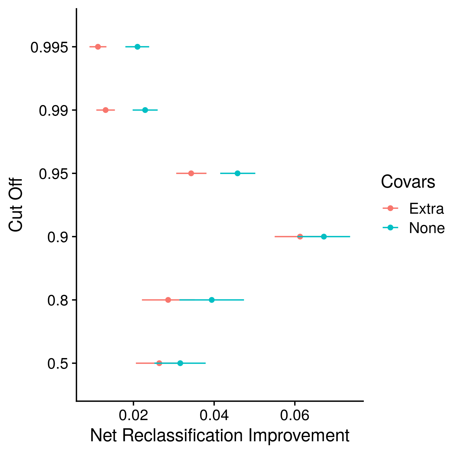
Figure 10.1: Example plot of the NRI
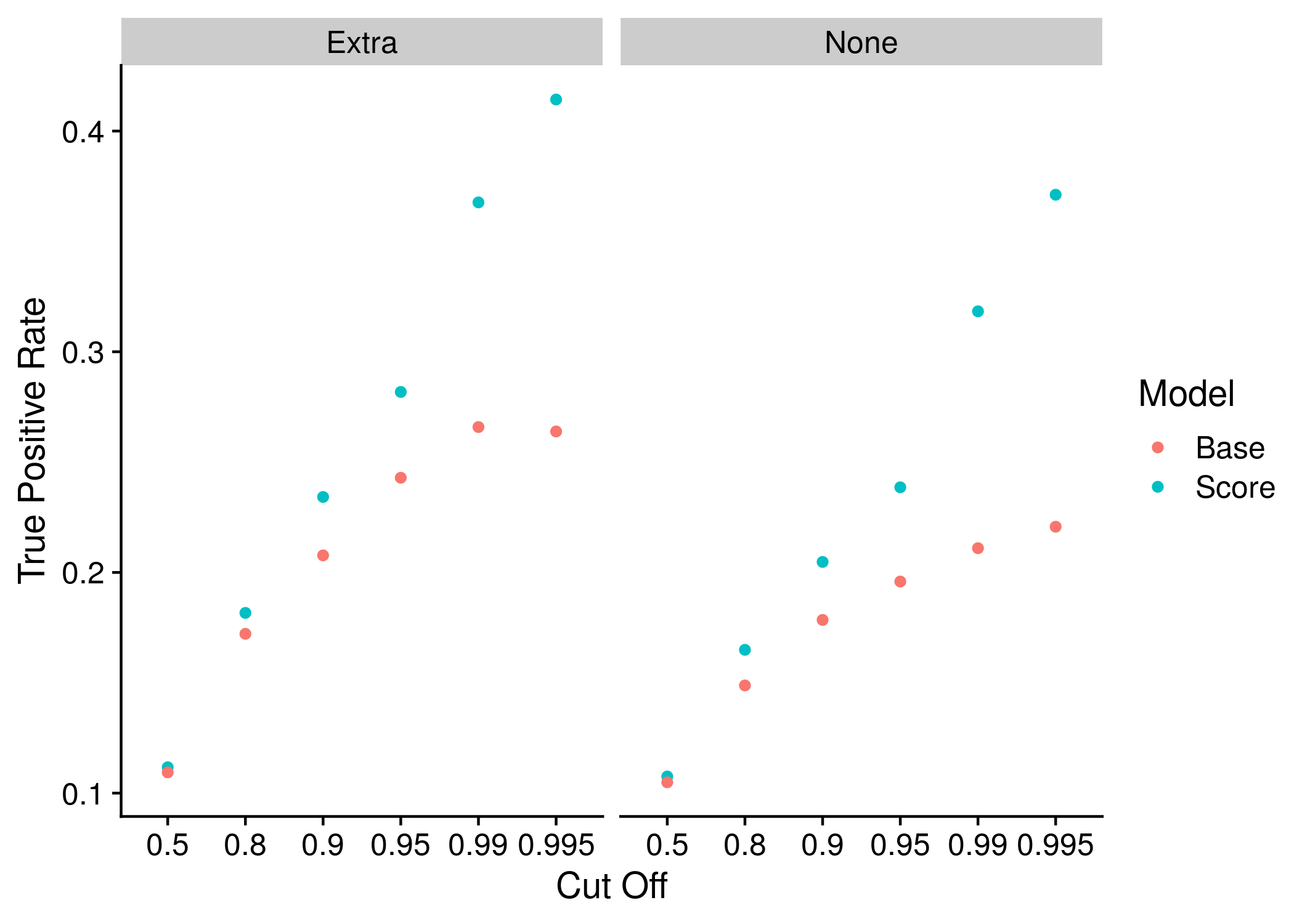
Figure 10.2: Example plot of the True Positive Rates
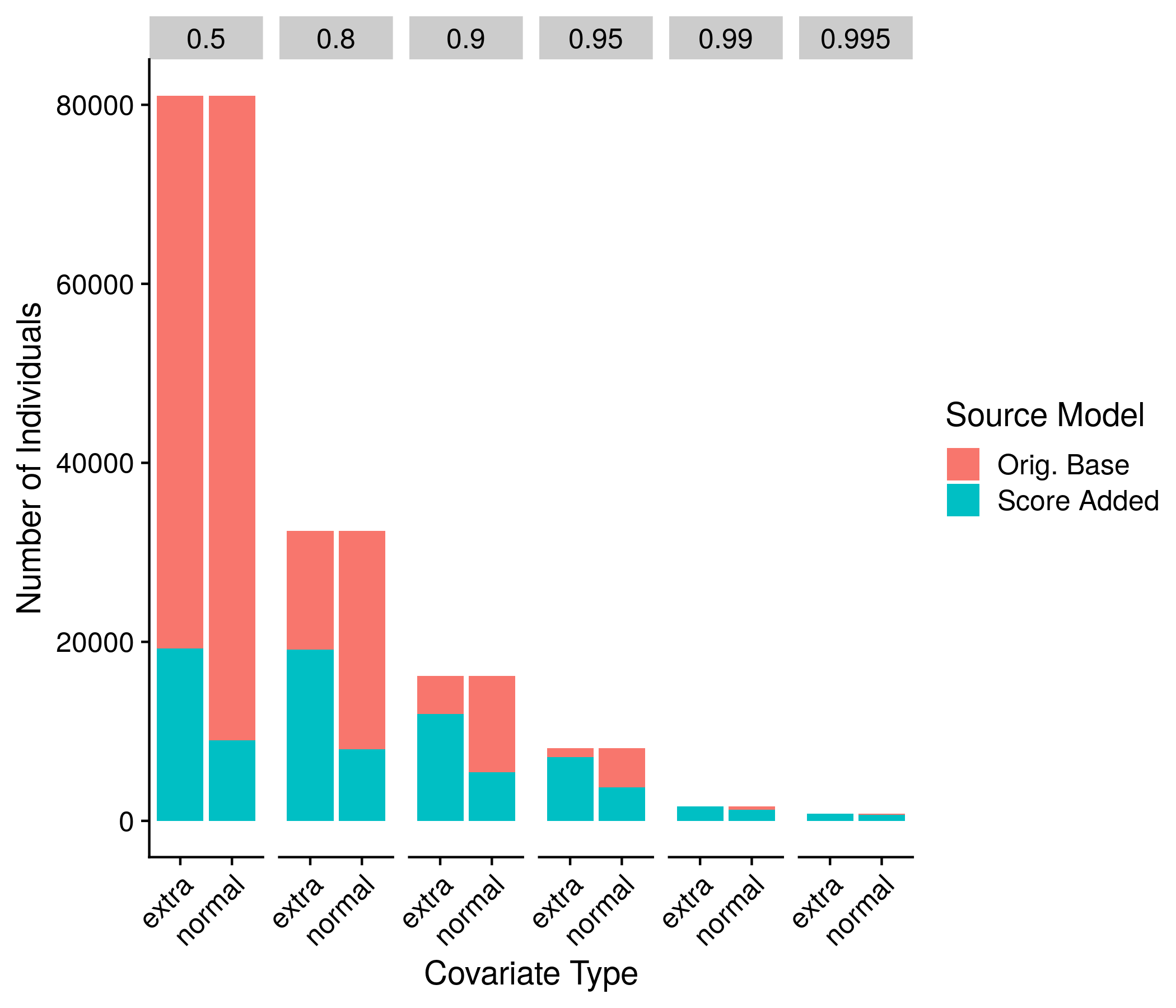
Figure 10.3: Example plot of the Reclassifications
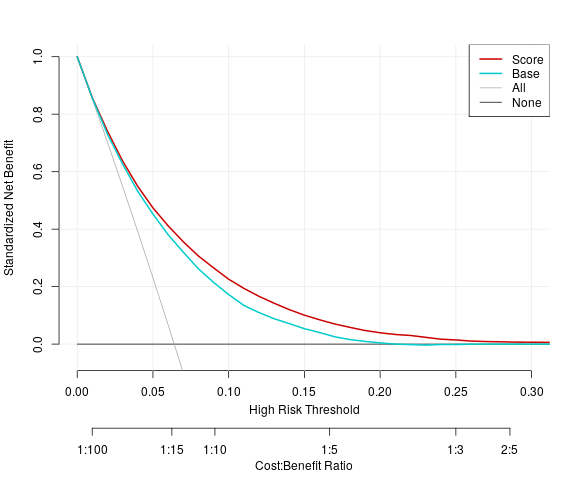
Figure 10.4: Example plot of the Decision Curve
And now the code:
library(stringr)
library(ggplot2)
library(cowplot)
library(pROC)
library(reshape2)
library(rmda)
theme_set(theme_cowplot())


convert_names <- function(x, the_dict = method_dict){
  y <- rep(NA, length(x))
  for(i in 1:length(x)){
    if(x[i] %in% the_dict[,1]){
      y[i] <- the_dict[the_dict[,1] == x[i], 2]
    }
  }
  return(y)
}

method_names <- read.table("local_info/method_names", stringsAsFactors = F)
disease_names <- read.table("local_info/disease_names", stringsAsFactors = F, sep = "\t")

all_authors <- unique(str_split(list.files("test_results/", "class_data"), "_", simplify = T)[,1])
if(any(all_authors == "Xie")){
  all_authors <- all_authors[-which(all_authors == "Xie")]
}


#in or out
full_count_in_out <- list()
full_pro_in_out <- list()
extra_full_count_in_out <- list()
extra_pro_in_out <- list()

#brier
brier_normal <- list()
brier_extra <- list()

#reclass
reclass_normal <- list()
reclass_extra <- list()

#rates
rates_normal <- list()
rates_extra <- list()

#true positive
tp_normal <- list()
tp_extra <- list()

#decision curves
dc_best_normal <- list()
dc_normal <- list()
dc_best_extra <- list()
dc_extra <- list()
dc_range_normal <- list()
dc_range_extra <- list()


for(author in all_authors){
  print(author)

  res <- readRDS(paste0("test_results/", author, "_class_data.RDS"))

  ################################################################################################
  #                                 IN OR OUT                                ####
  #################################################################################################

  plot_labels <- c("Number of Individuals", "Proportion of Individuals")
  for(opt in c("full", "pro")){

    #In or Out ####################################################
    risky_df <- data.frame(res[["score"]][["in_out"]])
    risky_df[,3] <- risky_df[,2] -  risky_df[,1]
    colnames(risky_df) <- c("intersect", "total", "diff")
    if(opt == "pro"){
      risky_df$intersect <- risky_df$intersect/risky_df$total
      risky_df$diff <- risky_df$diff/risky_df$total
    }
    risky_df$cut_off <- as.factor(c(0.5, 0.8, 0.9, 0.95, 0.99, 0.995))
    if(opt == "full"){
      full_count_in_out[[which(all_authors == author)]] <- risky_df[4,]
      full_count_in_out[[which(all_authors == author)]]$author <- author
    } else {
      full_pro_in_out[[which(all_authors == author)]] <- risky_df[4,]
      full_pro_in_out[[which(all_authors == author)]]$author <- author
    }
    risky_df <- melt(risky_df[,-2], id.vars = "cut_off")
    risky_df$type <- "normal"


    if(!is.null(res[["extra"]][[1]])){
      print("extra extra")
      extra_risky_df <- data.frame(res[["extra"]][["score"]][["in_out"]])
      extra_risky_df[,3] <- extra_risky_df[,2] -  extra_risky_df[,1]
      colnames(extra_risky_df) <- c("intersect", "total", "diff")
      if(opt == "pro"){
        extra_risky_df$intersect <- extra_risky_df$intersect/extra_risky_df$total
        extra_risky_df$diff <- extra_risky_df$diff/extra_risky_df$total
      }
      extra_risky_df$cut_off <- as.factor(c(0.5, 0.8, 0.9, 0.95, 0.99, 0.995))
      if(opt == "full"){
        extra_full_count_in_out[[which(all_authors == author)]] <- extra_risky_df[4,]
        extra_full_count_in_out[[which(all_authors == author)]]$author <- author
      } else {
        extra_pro_in_out[[which(all_authors == author)]] <- extra_risky_df[4,]
        extra_pro_in_out[[which(all_authors == author)]]$author <- author
      }
      extra_risky_df <- melt(extra_risky_df[,-2], id.vars = "cut_off")
      extra_risky_df$type <- "extra"

      plot_df <- rbind(extra_risky_df, risky_df)
      the_plot <- ggplot(plot_df, aes(type, value, fill = variable)) +
        geom_bar(stat="identity") +
        facet_grid( ~ cut_off) +
        labs(x = "Covariate Type", y = plot_labels[which(c("full", "pro") == opt)], fill = "Source Model") +
        scale_fill_discrete(labels = c("Orig. Base", "Score Added")) +
        theme(axis.text.x = element_text(angle = 45, vjust = 1, hjust=1))
      ggsave(paste0("addon_test_plots/", tolower(author), ".", opt, ".in_out.png"),
             the_plot, "png", height=6, width=7)

    } else {

      the_plot <- ggplot(risky_df, aes(cut_off, value, fill = variable)) + geom_bar(stat = "identity") +
        labs(x = "Cut Off", y = plot_labels[which(c("full", "pro") == opt)], fill = "Source Model") +
        scale_fill_discrete(labels = c("Orig. Base", "Score Added"))
      plot(the_plot)
      ggsave(paste0("addon_test_plots/", tolower(author), ".", opt, ".in_out.png"),
             the_plot, "png", height=6, width=7)
    }
  }


  ################################################################################################
  #                                 BRIER                               ####
  #################################################################################################
  brier_normal[[which(all_authors == author)]] <- c(res[["base"]][["brier"]], res[["score"]][["brier"]])
  if(!is.null(res[["extra"]][[1]])){
    brier_extra[[which(all_authors == author)]] <- c(res[["extra"]][["base"]][["brier"]],
                                                     res[["extra"]][["score"]][["brier"]])
  } else {
    brier_extra[[which(all_authors == author)]] <- c(NA, NA)
  }


  ################################################################################################
  #                                 RECLASS                              ####
  #################################################################################################

  #nri, idi
  reclass_df <- do.call("rbind", res[["score"]][["reclass"]])
  colnames(reclass_df) <- c("nri_est", "nri_lo", "nri_hi", "idi_est", "idi_lo", "idi_hi")
  reclass_df$cut_off <- as.factor(c(0.5, 0.8, 0.9, 0.95, 0.99, 0.995))

  reclass_normal[[which(all_authors == author)]] <- reclass_df
  reclass_normal[[which(all_authors == author)]]$disease <- convert_names(author, disease_names)

  reclass_df$stat <- "None"
  temp_df <- reclass_df


  if(!is.null(res[["extra"]][[1]])){
    reclass_df <- do.call("rbind", res[["extra"]][["score"]][["reclass"]])
    colnames(reclass_df) <- c("nri_est", "nri_lo", "nri_hi", "idi_est", "idi_lo", "idi_hi")
    reclass_df$cut_off <- as.factor(c(0.5, 0.8, 0.9, 0.95, 0.99, 0.995))

    reclass_extra[[which(all_authors == author)]] <- reclass_df
    reclass_extra[[which(all_authors == author)]]$disease <- convert_names(author, disease_names)

    reclass_df$stat <- "Extra"
    reclass_df <- rbind(reclass_df, temp_df)

    the_plot <- ggplot(reclass_df, aes(nri_est, cut_off, color = stat)) + geom_point() +
      geom_errorbar(aes(xmin = nri_lo, xmax = nri_hi, width = 0)) +
      labs(x = "Net Reclassification Improvement", y = "Cut Off", color = "Covars")
    plot(the_plot)
    ggsave(paste0("addon_test_plots/", tolower(author), ".nri.reclass.png"),
           the_plot, "png", height=5, width=5)

    the_plot <- ggplot(reclass_df, aes(idi_est, cut_off, color = stat)) + geom_point() +
      geom_errorbar(aes(xmin = idi_lo, xmax = idi_hi, width = 0)) +
      labs(x = "Integrated Discrimination Improvement", y = "Cut Off", color = "Covars")
    plot(the_plot)
    ggsave(paste0("addon_test_plots/", tolower(author), ".idi.reclass.png"),
           the_plot, "png", height=5, width=5)

  } else {
    reclass_extra[[which(all_authors == author)]] <- NULL

    the_plot <- ggplot(reclass_df, aes(nri_est, cut_off)) + geom_point() +
      geom_errorbar(aes(xmin = nri_lo, xmax = nri_hi, width = 0)) +
      labs(x = "Net Reclassification Improvement", y = "Cut Off")
    plot(the_plot)
    ggsave(paste0("addon_test_plots/", tolower(author), ".nri.reclass.png"),
           the_plot, "png", height=5, width=5)

    the_plot <- ggplot(reclass_df, aes(idi_est, cut_off)) + geom_point() +
      geom_errorbar(aes(xmin = idi_lo, xmax = idi_hi, width = 0)) +
      labs(x = "Integrated Discrimination Improvement", y = "Cut Off")
    plot(the_plot)
    ggsave(paste0("addon_test_plots/", tolower(author), ".idi.reclass.png"),
           the_plot, "png", height=5, width=5)

  }

  ################################################################################################
  #                                TPR FPR RATES                             ####
  #################################################################################################

  rate_df <- rbind(res[["score"]][["rates"]], res[["base"]][["rates"]],
                   res[["score"]][["rates"]] - res[["base"]][["rates"]])
  rate_df$type <- c("score", "base", "diff")
  rate_df$disease <- convert_names(author, disease_names)
  rates_normal[[which(all_authors == author)]] <- rate_df

  if(!is.null(res[["extra"]][[1]])){
    extra_rate_df <- rbind(res[["extra"]][["score"]][["rates"]], res[["extra"]][["base"]][["rates"]],
                     res[["extra"]][["score"]][["rates"]] - res[["extra"]][["base"]][["rates"]])
    extra_rate_df$type <- c("score", "base", "diff")
    extra_rate_df$disease <- convert_names(author, disease_names)
    rates_extra[[which(all_authors == author)]] <- extra_rate_df
  } else {
    rates_extra[[which(all_authors == author)]] <- NULL
  }

  ################################################################################################
  #                                TRUE POSITIVES                            ####
  #################################################################################################

  tp_df <-  as.data.frame(do.call("rbind", res[["score"]][["preds"]]))
  colnames(tp_df) <- c("score_tp", "total")
  tp_df$score_rate <- tp_df$score_tp/tp_df$total
  tp_df$base_tp <- do.call("rbind", res[["base"]][["preds"]])[,1]
  tp_df$base_rate <- tp_df$base_tp/tp_df$total
  tp_df$cut_off <- as.factor(c(0.5, 0.8, 0.9, 0.95, 0.99, 0.995))
  tp_df$disease <- convert_names(author, disease_names)


  plot_df <- data.frame("rate" = c(tp_df$score_rate, tp_df$base_rate, tp_df$score_rate - tp_df$base_rate),
                        "count" = c(tp_df$score_tp, tp_df$base_tp, tp_df$score_tp - tp_df$base_tp),
                        "type" = c(rep("Score", nrow(tp_df)), rep("Base", nrow(tp_df)), rep("diff", nrow(tp_df))),
                        "cut_off" = rep(tp_df$cut_off, 3),
                        "disease" = c(tp_df$disease, tp_df$disease, tp_df$disease))

  temp_df <- plot_df

  tp_normal[[which(all_authors == author)]] <- plot_df

  if(!is.null(res[["extra"]][[1]])){
    extra_tp_df <-  as.data.frame(do.call("rbind", res[["extra"]][["score"]][["preds"]]))
    colnames(extra_tp_df) <- c("score_tp", "total")
    extra_tp_df$score_rate <- extra_tp_df$score_tp/extra_tp_df$total
    extra_tp_df$base_tp <- do.call("rbind", res[["extra"]][["base"]][["preds"]])[,1]
    extra_tp_df$base_rate <- extra_tp_df$base_tp/extra_tp_df$total
    extra_tp_df$cut_off <- as.factor(c(0.5, 0.8, 0.9, 0.95, 0.99, 0.995))
    extra_tp_df$disease <- convert_names(author, disease_names)

    plot_df <- data.frame("rate" = c(extra_tp_df$score_rate, extra_tp_df$base_rate,
                                     extra_tp_df$score_rate - extra_tp_df$base_rate),
                          "count" = c(extra_tp_df$score_tp, extra_tp_df$base_tp,
                                      extra_tp_df$score_tp - extra_tp_df$base_tp),
                          "type" = c(rep("Score", nrow(extra_tp_df)), rep("Base", nrow(extra_tp_df)),
                                     rep("diff", nrow(extra_tp_df))),
                          "cut_off" = rep(extra_tp_df$cut_off, 3),
                          "disease" = c(extra_tp_df$disease, extra_tp_df$disease, extra_tp_df$disease))
    tp_extra[[which(all_authors == author)]] <- plot_df

    plot_df$ex <- "Extra"
    temp_df$ex <- "None"
    plot_df <- rbind(plot_df, temp_df)
    the_plot <- ggplot(plot_df[plot_df$type != "diff",], aes(cut_off, rate, color = type)) + geom_point() +
      labs(x = "Cut Off", y = "True Positive Rate", color = "Model") +
      facet_grid(cols = vars(ex))
    plot(the_plot)
    ggsave(paste0("addon_test_plots/", tolower(author), ".true_pos.png"),
           the_plot, "png", height=5, width=7)

  } else {
    tp_extra[[which(all_authors == author)]] <- NULL

    the_plot <- ggplot(plot_df[plot_df$type != "diff",], aes(cut_off, rate, color = type)) + geom_point() +
      labs(x = "Cut Off", y = "True Positive Rate", color = "Model")
    plot(the_plot)
    ggsave(paste0("addon_test_plots/", tolower(author), ".true_pos.png"),
           the_plot, "png", height=5, width=6)
  }


  ################################################################################################
  #                                DECISION CURVE                            ####
  #################################################################################################
  #plot_decision_curve(list(res[["score"]][["dc"]], res[["base"]][["dc"]]), curve.names = c("score", "base"))

  best_ind <- which.max(res[["score"]][["dc"]]$derived.data$sNB - res[["base"]][["dc"]]$derived.data$sNB)
  get_dc_df <- function(subres, the_ind){
    best_vals <- data.frame(t(c(subres[["base"]][["dc"]]$derived.data$sNB[the_ind],
                                subres[["score"]][["dc"]]$derived.data$sNB[the_ind])))
    colnames(best_vals) <- c("base", "score")
    best_vals$diff <- best_vals[1,2] - best_vals[1,1]
    best_vals$thresh <- subres[["score"]][["dc"]]$derived.data$thresholds[the_ind]
    best_vals$cb_ratio <- subres[["score"]][["dc"]]$derived.data$thresholds[the_ind]
    best_vals$just_nb <- subres[["score"]][["dc"]]$derived.data$NB[the_ind]
    return(best_vals)
  }

  get_dc_range <- function(subres){
    bool <- (subres[["score"]][["dc"]]$derived.data$sNB - subres[["base"]][["dc"]]$derived.data$sNB) > 0.001
    bool[is.na(bool)] <- FALSE
    better_range <- subres[["score"]][["dc"]]$derived.data$thresholds[bool]
    return(c(min(better_range), max(better_range)))
  }

  dc_range_normal[[which(all_authors == author)]] <- get_dc_range(res)
  dc_best_normal[[which(all_authors == author)]] <- get_dc_df(res, best_ind)
  dc_normal[[which(all_authors == author)]] <- rbind(get_dc_df(res, 2), get_dc_df(res, 6), get_dc_df(res, 13))
  png(paste0("addon_test_plots/", tolower(author), ".decision_curve.none.png"), width = 580, height = 480)
  plot_decision_curve(list(res[["score"]][["dc"]], res[["base"]][["dc"]]),
                     curve.names = c("Score", "Base"), xlim = c(0,0.3), confidence.intervals = F)
  dev.off()


  if(!is.null(res[["extra"]][[1]])){
    dc_range_extra[[which(all_authors == author)]] <- get_dc_range(res[["extra"]])
    best_ind <- which.max(res[["extra"]][["score"]][["dc"]]$derived.data$sNB -
                            res[["extra"]][["base"]][["dc"]]$derived.data$sNB)
    dc_best_extra[[which(all_authors == author)]] <- get_dc_df(res[["extra"]], best_ind)
    dc_extra[[which(all_authors == author)]] <- rbind(get_dc_df(res[["extra"]], 2),
                                                      get_dc_df(res[["extra"]], 6),
                                                      get_dc_df(res[["extra"]], 13))
    png(paste0("addon_test_plots/", tolower(author), ".decision_curve.extra.png"), width = 580, height = 480)
    plot_decision_curve(list(res[["extra"]][["score"]][["dc"]], res[["extra"]][["base"]][["dc"]]),
                      curve.names = c("score", "base"), xlim = c(0,0.3), confidence.intervals = F)
    dev.off()
  } else {
    dc_best_extra[[which(all_authors == author)]] <- NULL
    dc_extra[[which(all_authors == author)]] <- NULL
  }


}


#$$$$$$$$$$$$$$$$$$$$$$$$$$$$$$$$$$$$$$$$$$$$$$$$$$$$$$$$$$$$$$$$$$$$$$$$$$$$$$$$$$$$$$$$$$$$$$$
################################################################################################
#                                 OVERALL OVERALL OVERALL                                ####
#################################################################################################
#$$$$$$$$$$$$$$$$$$$$$$$$$$$$$$$$$$$$$$$$$$$$$$$$$$$$$$$$$$$$$$$$$$$$$$$$$$$$$$$$$$$$$$$$$$$$$$$$


################################################################################################
#                                 IN OR OUT                                ####
#################################################################################################

for(i in 1:length(all_authors)){
  if(is.null(extra_full_count_in_out[[i]])){
    extra_full_count_in_out[[i]] <- full_count_in_out[[i]]
    extra_pro_in_out[[i]] <- full_pro_in_out[[i]]
  }
}


plot_overall_in_out <- function(count_list, pro_list, covar_type, write_supp = FALSE){
  count_plot_df <- do.call("rbind", count_list)
  for_supp <- data.frame(count_plot_df)
  for_supp$disease <- convert_names(for_supp$author, disease_names)

  plot_df <- melt(count_plot_df, id.vars = c("author", "cut_off"))
  plot_df$disease <- convert_names(plot_df$author, disease_names)
  plot_df$disease <- factor(plot_df$disease,
                            levels = plot_df$disease[plot_df$variable == "diff"][order(plot_df$value[plot_df$variable == "diff"])])

  the_plot <- ggplot(plot_df[plot_df$variable != "total",], aes(value, disease, fill = variable)) +
    geom_bar(stat = "identity") +
    labs(x = "Number of Individuals", y = "", fill = "Source Model") +
    scale_fill_discrete(labels = c("Orig. Base", "Score Added"))
  plot(the_plot)
  ggsave(paste0("addon_test_plots/meta/in_out.count.", covar_type, ".png"),
         the_plot, "png", height=6, width=7)

  if(write_supp){
    plot_df <- plot_df[plot_df$variable != "total",c(5, 3, 4)]
    plot_df$diff <- plot_df$value[plot_df$variable == "diff"]
    plot_df <- plot_df[plot_df$variable != "diff",]
    colnames(plot_df) <- c("Disease", "x", "Orig. Base", "Score Added")
    write.table(plot_df[,-2], paste0("supp_tables/count.", covar_type, ".inout.txt"), row.names = F,
                col.names = T, sep = "\t", quote = F)
  }


  pro_plot_df <- do.call("rbind", pro_list)
  for_supp <- data.frame("disease" = for_supp$disease,
                         "count_new" = for_supp$diff, "count_intersect" = for_supp$intersect,
                         "pro_new" = pro_plot_df$diff, "pro_count" = pro_plot_df$intersect)
  write.table(for_supp, "supp_tables/in_out_all.txt", row.names = F, col.names = T, sep = "\t", quote = F)

  plot_df <- melt(pro_plot_df, id.vars = c("author", "cut_off"))
  plot_df$disease <- convert_names(plot_df$author, disease_names)
  plot_df$disease <- factor(plot_df$disease,
                            levels = plot_df$disease[plot_df$variable == "diff"][
                              order(plot_df$value[plot_df$variable == "diff"])])

  the_plot <- ggplot(plot_df[plot_df$variable != "total",], aes(value, disease, fill = variable)) +
    geom_bar(stat = "identity") +
    labs(x = "Proportion of Individuals", y = "", fill = "Source Model") +
    scale_fill_discrete(labels = c("Orig. Base", "Score Added"))
  plot(the_plot)
  ggsave(paste0("addon_test_plots/meta/in_out.pro.", covar_type, ".png"),
         the_plot, "png", height=6, width=7)

  if(write_supp){
    plot_df <- plot_df[plot_df$variable != "total",c(5, 3, 4)]
    plot_df$diff <- plot_df$value[plot_df$variable == "diff"]
    plot_df <- plot_df[plot_df$variable != "diff",]
    colnames(plot_df) <- c("Disease", "x", "Orig. Base", "Score Added")
    write.table(plot_df[,-2], paste0("supp_tables/pro.", covar_type, ".inout.txt"), row.names = F,
                col.names = T, sep = "\t", quote = F)
  }
}

plot_overall_in_out(full_count_in_out, full_pro_in_out, "norm", TRUE)
plot_overall_in_out(extra_full_count_in_out, extra_pro_in_out, "extra")


#*********************************************************************************
############################## FIGURE PLOT ########################################
#**********************************************************************************

pro_plot_df <- do.call("rbind", full_pro_in_out)
spec_author <- read.table("spec_authors", stringsAsFactors = F)


tp_df <- do.call("rbind", tp_normal)
tp_df <- tp_df[tp_df$cut_off == 0.95,]
tp_df <- tp_df[tp_df$type != "diff",]

plot_df <- melt(pro_plot_df, id.vars = c("author", "cut_off"))
plot_df$disease <- convert_names(plot_df$author, disease_names)
plot_df$disease <- factor(plot_df$disease,
                          levels = plot_df$disease[plot_df$variable == "diff"][
                            order(plot_df$value[plot_df$variable == "diff"])])

the_plot <- ggplot(plot_df[plot_df$variable != "total",], aes(value, disease, fill = variable)) +
  geom_bar(stat = "identity") +
  labs(x = "Proportion of Individuals", y = "", fill = "Source Model:") +
  scale_fill_discrete(labels = c("Base", "Score Incl.")) +
  theme(legend.position = "top")

i <- 1
tp_vars <- c("Score", "Base")
reclass_vars <- c("diff", "intersect")
for(curr_disease in levels(plot_df$disease)){
  for(j in 1:2){
    tp_val <- as.character(round(tp_df[tp_df$disease == curr_disease & tp_df$type == tp_vars[j], 1]*100, 1))
    if(j == 1){
      xpos <- plot_df[plot_df$disease == curr_disease & plot_df$variable == reclass_vars[j], 4]/2
    } else {
      xpos <- plot_df[plot_df$disease == curr_disease & plot_df$variable == reclass_vars[j-1], 4] +
              plot_df[plot_df$disease == curr_disease & plot_df$variable == reclass_vars[j], 4]/2
    }
    the_plot <- the_plot + annotate(geom = "text", label = tp_val, x = xpos, y = i, color = "white", size = 3)
  }
  i <- i + 1
}

plot(the_plot)
ggsave(paste0("addon_test_plots/meta/hopeful_fig.png"),
       the_plot, "png", height=6, width=7)


################################################################################################
#                                 BRIER                               ####
#################################################################################################

plot_brier <- function(brier_list, covar_type, write_supp = FALSE){
  brier_vals <- data.frame(do.call("rbind", brier_list))
  colnames(brier_vals) <- c("base", "score")
  brier_vals$diff <- brier_vals[,2] - brier_vals[,1]
  brier_vals$disease <- convert_names(all_authors, disease_names)
  brier_vals <- melt(brier_vals, id.vars = "disease")
  brier_vals$variable <- str_to_title(brier_vals$variable)

  brier_vals$disease <- factor(brier_vals$disease, unique(brier_vals$disease)[
    order(brier_vals$value[brier_vals$variable =="Score"])])
  the_plot <- ggplot(brier_vals[brier_vals$variable != "Diff",], aes(value, disease, color = variable)) +
    geom_point() + labs(x = "Brier Value", y = "", color = "Model")
  plot(the_plot)
  ggsave(paste0("addon_test_plots/meta/brier.", covar_type, ".png"),
         the_plot, "png", height=6, width=7)

  brier_vals$disease <- factor(brier_vals$disease, unique(brier_vals$disease)[
    order(brier_vals$value[brier_vals$variable =="Diff"])])
  the_plot <- ggplot(brier_vals[brier_vals$variable == "Diff",], aes(value, disease)) + geom_point() +
    labs(x = "Brier Value Diff.", y = "")
  plot(the_plot)

  if(write_supp){
    brier_vals <- data.frame("disease" = brier_vals$disease[brier_vals$variable == "Base"],
                             "Base" = signif(brier_vals$value[brier_vals$variable == "Base"], 3),
                             "Score" = signif(brier_vals$value[brier_vals$variable == "Score"], 3))
    write.table(brier_vals, "supp_tables/brier_vals.txt", quote = F, sep = "\t", col.names = T, row.names = F)
  }
}

plot_brier(brier_normal, "norm", TRUE)
plot_brier(brier_extra, "extra")

################################################################################################
#                                 RECLASS                              ####
#################################################################################################

plot_reclass <- function(reclass_list, covar_type, write_supp = FALSE){
  reclass_df <- do.call("rbind", reclass_list)

  reclass_df <- reclass_df[reclass_df$cut_off == 0.95,]

  reclass_df$disease <- factor(reclass_df$disease, levels = reclass_df$disease[order(reclass_df$nri_est)])
  the_plot <- ggplot(reclass_df, aes(nri_est, disease)) + geom_point() +
    labs(x = "Net Reclassification Improvement", y = "") +
    geom_errorbar(aes(xmin = nri_lo, xmax = nri_hi, width = 0))
  plot(the_plot)
  ggsave(paste0("addon_test_plots/meta/reclass.nri.", covar_type, ".png"),
         the_plot, "png", height=6, width=6)

  reclass_df$disease <- factor(reclass_df$disease, levels = reclass_df$disease[order(reclass_df$idi_est)])
  the_plot <- ggplot(reclass_df, aes(idi_est, disease)) + geom_point() +
    labs(x = "Integrated Discrimination Improvement", y = "") +
    geom_errorbar(aes(xmin = idi_lo, xmax = idi_hi, width = 0))
  plot(the_plot)
  ggsave(paste0("addon_test_plots/meta/reclass.idi.", covar_type, ".png"),
         the_plot, "png", height=6, width=6)

  if(write_supp){
    write.table(reclass_df[,c(8,1:3)], "supp_tables/nri_vals.txt", quote = F, sep = "\t", col.names = T, row.names = F)
    write.table(reclass_df[,c(8,4:6)], "supp_tables/idi_vals.txt", quote = F, sep = "\t", col.names = T, row.names = F)
  }
}


plot_reclass(reclass_normal, "norm", TRUE)
plot_reclass(reclass_extra, "extra")

pval_reclass <- do.call("rbind", reclass_normal)
pval_reclass <- pval_reclass[pval_reclass$cut_off == 0.95,]


################################################################################################
#                                 TPR FPR RATES                            ####
#################################################################################################

plot_rates <- function(rates_list, covar_type, write_supp = FALSE){
  rate_vals <- data.frame(do.call("rbind", rates_list))
  rate_vals <- melt(rate_vals, id.vars = c("type", "disease"))

  rate_vals$disease <- factor(rate_vals$disease, levels = unique(rate_vals$disease)[
    order(rate_vals$value[rate_vals$variable == "tpr" & rate_vals$type == "score"])])
  rate_vals$type <- str_to_title(rate_vals$type)
  the_plot <- ggplot(rate_vals[rate_vals$type != "Diff" & rate_vals$variable == "tpr",],
                     aes(value, disease, color = type)) + geom_point() +
    labs(x = "True Positive Rate", y = "", color = "Model")
  plot(the_plot)
  ggsave(paste0("addon_test_plots/meta/tpr.", covar_type, ".png"),
         the_plot, "png", height=6, width=6)

  rate_vals$disease <- factor(rate_vals$disease, levels = unique(rate_vals$disease)[
    order(rate_vals$value[rate_vals$variable == "tpr" & rate_vals$type == "Diff"])])
  the_plot <- ggplot(rate_vals[rate_vals$type == "Diff" & rate_vals$variable == "tpr",],
                     aes(value, disease)) + geom_point() +
    labs(x = "True Positive Rate Diff.", y = "")
  plot(the_plot)

  if(write_supp){
    write_df <- data.frame("disease" = rate_vals$disease[rate_vals$type == "Score" & rate_vals$variable == "fpr"],
                           "TPR - Base" = signif(rate_vals$value[rate_vals$type == "Base" & rate_vals$variable == "tpr"], 3),
                           "FPR - Base" = signif(rate_vals$value[rate_vals$type == "Base" & rate_vals$variable == "fpr"], 3),
                           "TPR - Score" = signif(rate_vals$value[rate_vals$type == "Score" & rate_vals$variable == "tpr"], 3),
                           "FPR - Score" = signif(rate_vals$value[rate_vals$type == "Score" & rate_vals$variable == "fpr"], 3))
    write.table(write_df, "supp_tables/tpr_fpr_vals.txt", quote = F, sep = "\t", col.names = T, row.names = F)

  }
}

plot_rates(rates_normal, "norm", TRUE)
plot_rates(rates_extra, "extra")


################################################################################################
#                                 TRUE POSITIVES                          ####
#################################################################################################

plot_tp <- function(tp_list, covar_type){
  tp_df <- do.call("rbind", tp_list)
  tp_df <- tp_df[tp_df$cut_off == 0.95,]
  tp_df$type <- str_to_title(tp_df$type)
  tp_df$disease <- factor(tp_df$disease, levels = unique(tp_df$disease)[order(tp_df$rate[tp_df$type == "Diff"])])
  the_plot <- ggplot(tp_df[tp_df$type == "Diff",], aes(rate, disease)) + geom_point() +
    labs(x = "True Positive Rate Diff.", y = "")
  plot(the_plot)

  tp_df$disease <- factor(tp_df$disease, levels = unique(tp_df$disease)[order(tp_df$rate[tp_df$type == "Score"])])
  the_plot <- ggplot(tp_df[tp_df$type != "Diff",], aes(rate, disease, color = type)) + geom_point() +
    labs(x = "True Positive Rate", y = "", color = "Model")
  plot(the_plot)
  ggsave(paste0("addon_test_plots/meta/risky_tp.", covar_type, ".png"),
         the_plot, "png", height=6, width=6)
}

plot_tp(tp_normal, "norm")
plot_tp(tp_extra, "extra")
exit()

df <- do.call("rbind", tp_normal)
x <- df[df$cut_off == 0.95 & df$type == "Score",]
y <- df[df$cut_off == 0.95 & df$type == "Base",]

supp_df <- data.frame("disease" = df[df$type == "Score" & df$cut_off == 0.95,5],
                      "Base" = signif(df[df$type == "Base" & df$cut_off == 0.95,1], 3),
                      "Score" = signif(df[df$type == "Score" & df$cut_off == 0.95,1], 3))
write.table(supp_df, "supp_tables/simple_tp.txt", row.names = F, col.names = T, quote = F, sep = "\t")

################################################################################################
#                                 DECISION CURVES                         ####
#################################################################################################

dc_plot <- function(dc_best, dc_all, dc_range, cov_type, write_supp = FALSE){
  disease_bool <- unlist(lapply(dc_best, function(x) x$thresh != 0))
  new_disease_names <- convert_names(all_authors, disease_names)[disease_bool]

  dc_df <- do.call("rbind", dc_best)
  dc_df <- dc_df[disease_bool,]
  dc_df$disease <- new_disease_names
  dc_df <- dc_df[dc_df$score != 1,]
  dc_df <- melt(dc_df, id.vars = c("thresh", "cb_ratio", "disease"))

  dc_df$disease <- factor(dc_df$disease, levels = unique(dc_df$disease)[order(dc_df$value[dc_df$variable == "score"])])
  dc_df$variable <- str_to_title(dc_df$variable)
  dc_df$variable[dc_df$variable == "Base"] <- "Base"
  dc_df$variable[dc_df$variable == "Score"] <- "Score Incl."
  the_plot <- ggplot(dc_df[dc_df$variable %in% c("Base", "Score Incl."),], aes(value, disease, color = variable)) + geom_point() +
    labs(x = "Standardized Net Benefit", y = "", color = "Model:") +
    theme(legend.position = "top",  legend.text = element_text(size = 10))

  plot(the_plot)
  ggsave(paste0("addon_test_plots/meta/dc.best.", cov_type, ".png"),
         the_plot, "png", height=6, width=4.5)

  if(write_supp){
    write_df <- dc_df[dc_df$variable != "Diff",]
    write_df <- data.frame("disease" = write_df$disease[write_df$variable == "Base"],
                           "Base NB" = signif(write_df$value[write_df$variable == "Base"],3),
                           "Base Thresh" = write_df$thresh[write_df$variable == "Base"],
                           "Score NB" = signif(write_df$value[write_df$variable == "Score Incl."],3),
                           "Score Thresh" = write_df$thresh[write_df$variable == "Score Incl."])
    write.table(write_df, "supp_tables/dc_best.txt", quote = F, sep = "\t", col.names = T, row.names = F)
  }


  dc_df <- do.call("rbind", dc_all)
  dc_df$disease <- rep(convert_names(all_authors, disease_names), each = 3)
  dc_df <- dc_df[dc_df$score != 1,]
  dc_df <- melt(dc_df, id.vars = c("thresh", "cb_ratio", "disease"))

  dc_df$disease <- factor(dc_df$disease, levels = unique(dc_df$disease)[
    order(dc_df$value[dc_df$variable == "score" & dc_df$thresh == 0.05])])
  dc_df$variable <- str_to_title(dc_df$variable)
  dc_df$variable[dc_df$variable == "Base"] <- "Base"
  dc_df$variable[dc_df$variable == "Score"] <- "Score Incl."
  dc_df$thresh <- paste0("Thresh. = ", dc_df$thresh)
  the_plot <- ggplot(dc_df[dc_df$variable %in% c("Base", "Score Incl."),], aes(value, disease, color = variable)) + geom_point() +
    labs(x = "Standardized Net Benefit", y = "", color = "Model:") +
    facet_grid(cols = vars(thresh)) + theme(legend.position = "top")
  plot(the_plot)
  ggsave(paste0("addon_test_plots/meta/dc.many.", cov_type, ".png"),
         the_plot, "png", height=6, width=8)

  if(write_supp){
    write_df <- dc_df[dc_df$variable != "Diff",]
    write_df <- data.frame("disease" = write_df$disease[write_df$variable == "Base" & write_df$cb_ratio == 0.01],
                           "Base NB - 0.01" = signif(write_df$value[write_df$variable == "Base" & write_df$cb_ratio == 0.01],3),
                           "Base NB - 0.05" = signif(write_df$value[write_df$variable == "Base" & write_df$cb_ratio == 0.05],3),
                           "Base NB - 0.12" = signif(write_df$value[write_df$variable == "Base" & write_df$cb_ratio == 0.12],3),
                           "Score NB - 0.01" = signif(write_df$value[write_df$variable == "Score Incl." & write_df$cb_ratio == 0.01],3),
                           "Score NB - 0.05" = signif(write_df$value[write_df$variable == "Score Incl." & write_df$cb_ratio == 0.05],3),
                           "Score NB - 0.12" = signif(write_df$value[write_df$variable == "Score Incl." & write_df$cb_ratio == 0.12],3))
    write.table(write_df, "supp_tables/dc_all.txt", quote = F, sep = "\t", col.names = T, row.names = F)
  }


  dc_range <- data.frame(do.call("rbind", dc_range))
  colnames(dc_range) <- c("start", "end")
  dc_range <- dc_range[disease_bool,]
  dc_range$disease <- new_disease_names
  #dc_range <- dc_range[!is.infinite(dc_range[,1]),]
  dc_range$disease <- factor(dc_range$disease, levels = dc_range$disease[order(dc_range$end - dc_range$start)])
  the_plot <- ggplot(dc_range, aes(start, disease)) + geom_point(size = 0) +
    geom_errorbarh(aes(xmin = start, xmax = end, height = 0)) +
    labs(x = "Positive Net Benefit Threshold", y = "")
  plot(the_plot)
  ggsave(paste0("addon_test_plots/meta/dc.range.", cov_type, ".png"),
         the_plot, "png", height=6, width=6)

  dc_df$thresh[dc_df$thresh == "Thresh. = 0.05"] <- "Thresh. = 95%"
  dc_df$thresh[dc_df$thresh == "Thresh. = 0.01"] <- "Thresh. = 99%"
  dc_df$thresh[dc_df$thresh == "Thresh. = 0.12"] <- "Thresh. = 88%"
  dc_df <- dc_df[dc_df$disease %in% dc_range$disease[(dc_range$end - dc_range$start) > 0.10],]
  the_plot <- ggplot(dc_df[dc_df$variable %in% c("Base", "Score Incl."),], aes(value, disease, color = variable)) + geom_point() +
    labs(x = "Standardized Net Benefit", y = "", color = "Model:") +
    facet_grid(cols = vars(thresh)) + theme(legend.position = "top")
  plot(the_plot)
  ggsave(paste0("addon_test_plots/meta/dc.for_fig.", cov_type, ".png"),
         the_plot, "png", height=3.8, width=8)

  if(write_supp){
    write_df <- dc_range
    write.table(write_df, "supp_tables/dc_range.txt", quote = F, sep = "\t", col.names = T, row.names = F)
  }
}

dc_plot(dc_best_normal, dc_normal, dc_range_normal, "norm", TRUE)
dc_plot(dc_best_extra, dc_extra, dc_range_extra, "extra")

ex <- do.call("rbind", dc_best_extra)
norm <- do.call("rbind", dc_best_normal)
ex <- ex[ex[,1] != 1,]
norm <- norm[norm[,1] != 1 & unlist(lapply(dc_best_extra, function(x) !is.null(x))),]

write_df <- data.frame(convert_names(all_authors, disease_names), matrix(0, nrow = 23, ncol = 4))
j=1
for(i in 1:23){
    write_df[i,j+2] <- signif(dc_best_normal[[i]]$base, 3)
    write_df[i,j+1] <- signif(dc_best_normal[[i]]$score, 3)
    if(!is.null(dc_best_extra[[i]])){
      write_df[i,j+4] <- signif(dc_best_extra[[i]]$base, 3)
      write_df[i,j+3] <- signif(dc_best_extra[[i]]$score, 3)
    }
}
write_df <- write_df[write_df[,2] != 1,]
colnames(write_df) <- c("Disease", "Score-No", "Base-No", "Score-Extra", "Base-Extra")
write.table(write_df, "supp_tables/dc_extra.txt", row.names = F, col.names = T, quote = F, sep = '\t')