12 To Do

12.1 Across Score Evaluations

Now I will describe evaluaitons that are only possible when comparing multiple scores to each other.

12.1.1 Set-Up

The goal of the set-up is not to analyze the polygenic risk score itself (a value for every person), but rather a series of statistics/values that correspond to each score. Therefore, our final product from this set-up is a data frame with each row containing a score and each column containing a statistic/value. We can seperate these columns into different classes. The first class related to predictive performance, namely AUC and its CI. The second class involves the score but is nonpredictive, including number of SNPs, phenotype and parameter. The find class involves the phenotpe at large, including heritability, number of SNPs in the summary statistics, case/control information, and similar information. This large data frame is finally subset into smaller datasets that only contain the best score at-large or the best score for each type of method within a given phenotype. These data frames fuel the later analyses,

We construct this all-important data frame by iterating rhough each author (or disease) under analysis. For each author we read in the AUC, the the case/control split of UKBB, and the number of SNPs each score. We assign each piece of data to an element of a list, and after the for loop combine everything together. Lastly, we read in meta-statistics generated back from when we refined the raw summary statistics. We then add the meta-statistics for each author to the corresponding row. The exact code is:

#When all of the tuning is done want to go though and check that 
#If method performance is dependent on any factors (sample size, SNPs, etc.)
  #Do for one AUC for each author (the best)
  #Do this once for each method (the best method for each author)

#Want to see if there is a correlation between method parameters and the meta stats
  #so collect all results (for all authors) then run a model

#Also want to compare training to testing results

#Will focus on AUC

splitter <- function(values, N){
  inds = c(0, sapply(1:N, function(i) which.min(abs(cumsum(as.numeric(values)) - sum(as.numeric(values))/N*i))))
  dif = diff(inds)
  if(any(dif == 0)){
    dif[1] <- dif[1] - sum(dif == 0)
    dif[dif == 0] <- 1
  }

  re = rep(1:length(dif), times = dif)
  return(split(values, re))
}


options(warn = 2)

list_all_auc <- list()
list_all_best_names <- list()
list_all_best_methods <- list()
list_ukb_cc <- list()
list_ukb_snps <- list()
list_ukb_beta_pdiff <- list()
list_ukb_len_pdiff <- list()
list_pval_6 <- list()
list_pval_8 <- list()
list_beta_len <- list()
list_beta_effect <- list()



i <- 1
all_author <- unlist(lapply(strsplit(list.files("../tune_score/tune_results/", "res"), "_"), function(x) x[1]))
all_author <- all_author[all_author != "Xie"]
for(author in all_author){
  all_res <- readRDS(paste0("../tune_score/tune_results/", author, "_res.RDS"))
  score_names <- all_res[["score_names"]]

  #GWAS Stats
  orig_gwas <- read.table(paste0("~/athena/doc_score/raw_ss/", author, "/clean_", tolower(author), ".txt.gz"), stringsAsFactors=F, header=T)
  four_len <- unlist(lapply(splitter(sort(abs(orig_gwas$BETA[orig_gwas$P < 0.05])), 4), function(x) length(x)))
  four_mean <- unlist(lapply(splitter(sort(abs(orig_gwas$BETA[orig_gwas$P < 0.05])), 4), function(x) mean(x)))
  list_beta_len[[i]] <- (four_len[4] - four_len[1])/four_len[1]
  list_beta_effect[[i]] <- (four_mean[4] - four_mean[1])/four_mean[1]
  list_pval_6[[i]] <- sum(orig_gwas$P < 1e-6)
  list_pval_8[[i]] <- sum(orig_gwas$P < 1e-8)

  #read in
  list_all_best_names[[i]] <- read.table(paste0("../tune_score/tune_results/", tolower(author), ".best.ss"), stringsAsFactors=F)
  list_all_best_methods[[i]] <- read.table(paste0("../tune_score/tune_results/", tolower(author), ".methods.ss"), stringsAsFactors=F)

  #get the mean_auc, and put in other info
  mean_auc <- as.data.frame(Reduce("+", all_res[["auc"]])/length(all_res[["auc"]]))
  mean_auc$name <- score_names
  mean_auc$method <- unlist(lapply(strsplit(score_names, ".", fixed=T), function(x) x[3]))
  mean_auc$author <- author

  #get the case control in UKBB
  ukb_pheno <- read.table(paste0("../construct_defs/pheno_defs/diag.", tolower(author) ,".txt.gz"), stringsAsFactors=F)
  list_ukb_cc[[i]] <- t(matrix(as.numeric(table(rowSums(ukb_pheno[,1:4]) > 0))))[rep(1, nrow(mean_auc)),]

  #get the ukb snp lengths
  ukb_snps <- rep(0, nrow(list_all_best_methods[[i]]))
  ukb_beta_pdiff <- rep(0, nrow(list_all_best_methods[[i]]))
  ukb_len_pdiff <- rep(0, nrow(list_all_best_methods[[i]]))
  for(sname in list_all_best_methods[[i]][,1]){
    new_name <- paste0(strsplit(sname, ".", fixed = T)[[1]][3], ".", strsplit(sname, ".", fixed = T)[[1]][2], ".ss.gz")
    get_files <- list.files(paste0("../../mod_sets/", author, "/"), pattern = new_name)
    prs_sets <- list()
    #temp_length <- rep(0, length(get_files))
    for(j in 1:length(get_files)){
      #temp_length[j] <- as.numeric(system(paste0("cat ../../mod_sets/", author, "/", get_files[j], " | wc -l"), intern = TRUE))
      prs_sets[[j]] <- read.table(paste0("../../mod_sets/", author, "/", get_files[j]), stringsAsFactors=F, header=T)
      colnames(prs_sets[[j]]) <- paste0(rep("X", ncol(prs_sets[[j]])), 1:ncol(prs_sets[[j]]))
    }
    prs_sets <- do.call("rbind", prs_sets)

    ukb_snps[which(list_all_best_methods[[i]][,1] == sname)] <- nrow(prs_sets)
    if(length(unique(prs_sets[,7])) > 10){
      temp <- unlist(lapply(splitter(sort(abs(sort(prs_sets[,7]))), 4), function(x) mean(x)))
      ukb_beta_pdiff[which(list_all_best_methods[[i]][,1] == sname)] <- (temp[4] - temp[1])/temp[1]
      temp <- unlist(lapply(splitter(sort(abs(sort(prs_sets[,7]))), 4), function(x) length(x)))
      ukb_len_pdiff[which(list_all_best_methods[[i]][,1] == sname)] <- (temp[4] - temp[1])/temp[1]
    } else {
      ukb_beta_pdiff[which(list_all_best_methods[[i]][,1] == sname)] <- NA
      ukb_len_pdiff[which(list_all_best_methods[[i]][,1] == sname)] <- NA
    }
  }

  names(ukb_snps) <- list_all_best_methods[[i]][,1]
  list_ukb_snps[[i]] <- ukb_snps
  list_ukb_beta_pdiff[[i]] <- ukb_beta_pdiff
  list_ukb_len_pdiff[[i]] <- ukb_len_pdiff


  list_all_auc[[i]] <- mean_auc
  i <- i + 1
}

for(i in 1:length(list_pval_6)){
  list_pval_6[[i]] <- rep(list_pval_6[[i]], length(list_ukb_snps[[i]]))
  list_pval_8[[i]] <- rep(list_pval_8[[i]], length(list_ukb_snps[[i]]))
  list_beta_len[[i]] <- rep(list_beta_len[[i]], length(list_ukb_snps[[i]]))
  list_beta_effect[[i]] <- rep(list_beta_effect[[i]], length(list_ukb_snps[[i]]))
}


#add meta info to the all_auc
all_auc <- do.call("rbind", list_all_auc)
all_auc <- cbind(all_auc, do.call("rbind", list_ukb_cc))

method_best_names <- unlist(list_all_best_methods)
all_auc <- all_auc[all_auc$name %in% method_best_names,]
all_auc <- cbind(all_auc, unlist(list_ukb_snps), unlist(list_ukb_beta_pdiff), unlist(list_ukb_len_pdiff), unlist(list_pval_6), unlist(list_pval_8), unlist(list_beta_len), unlist(list_beta_effect))

colnames(all_auc) <- c("auc_lo", "auc", "auc_hi", "name", "method", "author", "uk_control", "uk_case", "uk_snps", "uk_beta_pdiff", "uk_len_pdiff", "sig6_gwas_snps", "sig8_gwas_snps", "len_pdiff", "effect_pdiff")

meta_info <- read.table("../../raw_ss/meta_stats", stringsAsFactors=F, sep=",", header=T)
add_on <- data.frame(matrix(0, nrow = nrow(all_auc), ncol = 10))
colnames(add_on) <- colnames(meta_info)[-c(1,2)]
for(author in unique(all_auc$author)){
  add_on[all_auc$author == author,] <- meta_info[meta_info$author == author,-c(1,2)]
}
all_auc <- cbind(all_auc, add_on)

all_auc$uk_cc_ratio <- all_auc$uk_case/all_auc$uk_control
all_auc$gwas_cc_ratio <- all_auc$cases/all_auc$controls
all_auc$uk_sampe_size <- all_auc$uk_case + all_auc$uk_control

#get the best names (absolute best, and best name for each method for each author)
abs_best_names <- unlist(lapply(list_all_best_names, function(x) x[3,2]))

for(reg_name in c("uk_snps", "uk_beta_pdiff", "uk_len_pdiff", "sig6_gwas_snps", "sig8_gwas_snps", "len_pdiff", "effect_pdiff", "sampe_size", "snps", "h2", "uk_cc_ratio", "gwas_cc_ratio")){
  all_auc[reg_name] <- (all_auc[reg_name] - min(all_auc[reg_name], na.rm=T))/(max(all_auc[reg_name],na.rm=T) - min(all_auc[reg_name],na.rm=T))
}

#subset the all_auc
all_auc$ancestry <- as.numeric(as.factor(all_auc$ancestry))
all_auc <- all_auc[,-which(colnames(all_auc) %in% c("ldsc_h2", "ldsc_h2_se", "hdl_h2", "hdl_h2_se", "hdl_h2se"))]
abs_best_auc <- all_auc[all_auc$name %in% abs_best_names,]
method_best_auc <- all_auc

12.1.2 Meta Info Regressions

With all of the data prepared we go go onto actually conducting the regressions. This section is actually relatively simple as all we have to do is call a lm command for each meta-statistic as the independent variable. To further break things down, the data I am pulling from in each regression is broken into the best method for each disease, or the best parameter-set for a given method for each disease. I am therefore able to estimate not only the overall impact of the number of initial SNPs (for example) on performance, but also whether this effect of number of SNPs only applies to the clumping method. After each regression I keep the regression coefficent, standard error, z-value and p-value. The exact code is:

############################################################
################ META INFO REGRESSIONS #####################
############################################################

meta_to_regress <- c("uk_snps", "uk_beta_pdiff", "uk_len_pdiff", "sig6_gwas_snps", "sig8_gwas_snps", "len_pdiff", "effect_pdiff", "sampe_size", "ancestry", "snps", "h2", "uk_cc_ratio", "gwas_cc_ratio")
abs_best_coefs <- matrix(0, nrow = length(meta_to_regress), ncol = 4)
all_poss_coefs <- matrix(0, nrow = length(meta_to_regress), ncol = 4)
method_best_coefs <- rep(list(matrix(0, nrow = length(meta_to_regress), ncol = 4)), length(unique(method_best_auc$method)))

for(i in 1:length(meta_to_regress)){
  best_mod <- lm(as.formula(paste0("auc ~ ", meta_to_regress[i])), data = abs_best_auc)
  abs_best_coefs[i,] <- summary(best_mod)$coefficients[2,]

  all_mod <- lm(as.formula(paste0("auc ~ ", meta_to_regress[i])), data = method_best_auc)
  all_poss_coefs[i,] <- summary(all_mod)$coefficients[2,]

  for(m in unique(method_best_auc$method)){
     method_mod <- lm(as.formula(paste0("auc ~ ", meta_to_regress[i])), data = method_best_auc[method_best_auc$method == m,])
     method_best_coefs[[which(unique(method_best_auc$method) == m)]][i,] <- summary(method_mod)$coefficients[2,]
  }
}


#should add regressions across all for best method, not just abs best auc
meta_to_regress <- meta_to_regress[-which(meta_to_regress == "ancestry")]
umethod <- unique(method_best_auc$method)
method_holder <- data.frame(matrix(0, nrow = length(meta_to_regress)*2, ncol = length(umethod)))
norm_auc <- (method_best_auc$auc - min(method_best_auc$auc))/(max(method_best_auc$auc) - min(method_best_auc$auc))
k <- 1
for(i in 1:length(meta_to_regress)){
  j <- which(colnames(method_best_auc) == meta_to_regress[i])
  stat_val <- (method_best_auc[,j] - min(method_best_auc[,j]))/(max(method_best_auc[,j]) - min(method_best_auc[,j]))
  temp <- method_best_auc[order(norm_auc*stat_val,decreasing=T),]
  top_method <- temp$method[!duplicated(temp$author)][1:10]

  for(m in unique(top_method)){
    method_holder[k,which(umethod == m)] <- sum(top_method == m)
  }

  stat_val <- abs(stat_val - 1)
  temp <- method_best_auc[order(norm_auc*stat_val,decreasing=T),]
  top_method <- temp$method[!duplicated(temp$author)][1:10]

  for(m in unique(top_method)){
    method_holder[k+1,which(umethod == m)] <- sum(top_method == m)
  }

  k <- k + 2
}

colnames(method_holder) <- umethod
method_holder$stat <- paste0(c("", "rev_"), rep(meta_to_regress, each=2))

12.1.3 Testing and Training Comparison

While not the main objective of determining whether meta-statistic effect the performance of polygenic risk scores, comparing training and testing accuracies is an important step to determine model overfitting. For example, if the AUC is very high in training compared to testing then we know the cross validation in the training step did not adequately lead to independent groups and perhaps the entire assessment of best scores could be corrputed. The process to check this problem is luckily quite simple. We simply read in the training and testing results, average over the folds in the training group, then take the difference between each. The exact code is shown below (including the final step of saving everything):

############################################################
################ TRAIN AND TEST COMP #####################
############################################################

ttcomp <- matrix(0, nrow = length(all_author), ncol = 4)

k <- 1
for(author in all_author){
  tune_res <- readRDS(paste0("../tune_score/tune_results/", author, "_res.RDS"))
  test_res <- readRDS(paste0("../test_score/final_stats/", author, "_res.RDS"))
  use_name <- test_res[["score_names"]]
  use_index <- which(tune_res[["score_names"]] == use_name)

  mean_conc <- Reduce("+", tune_res[["conc"]])/length(tune_res[["conc"]])
  mean_auc <- Reduce("+", tune_res[["auc"]])/length(tune_res[["auc"]])
  mean_or <- Reduce("+", tune_res[["or"]])/length(tune_res[["or"]])
  mean_survfit <- matrix(0, nrow = length(tune_res[["survfit"]][[1]]), ncol = 6)
  for(i in 1:length(tune_res[["survfit"]])){
    for(j in 1:length(tune_res[["score_names"]])){
      mean_survfit[j,] <- mean_survfit[j,] + as.numeric(tune_res[["survfit"]][[i]][[j]])
    }
  }
  mean_survfit <- mean_survfit/length(tune_res[["survfit"]])

  mean_conc <- mean_conc[use_index,]
  mean_auc <- mean_auc[use_index,]
  mean_or <- mean_or[use_index,]
  mean_survfit <- mean_survfit[use_index,]

  diff_conc <- as.numeric(test_res[["conc"]][1] - mean_conc[1])
  diff_auc <- test_res[["auc"]][[2]][2] - mean_auc[2]
  diff_or <- test_res[["or"]][2,2] - mean_or[2]
  diff_survfit <- test_res[["survfit"]][nrow(test_res[["survfit"]]),3] - mean_survfit[2]


  ttcomp[k,] <- c(diff_conc, diff_survfit, diff_auc, diff_or)
  k <- k + 1
}

12.1.4 Plotting

The seperated plotting process is nicely, quite simple. We first create plots to show the effect and standard error of each regression (straightforward seemingly obvious thing to do). To spice thing up we also make two plots to show some of the more interesting correlations between the meta-statistics and significances therein. Lastly, we plot the training and testing differences through a simple dot plot. Seeing as everything is simple enough I will stop now and leave the code below:

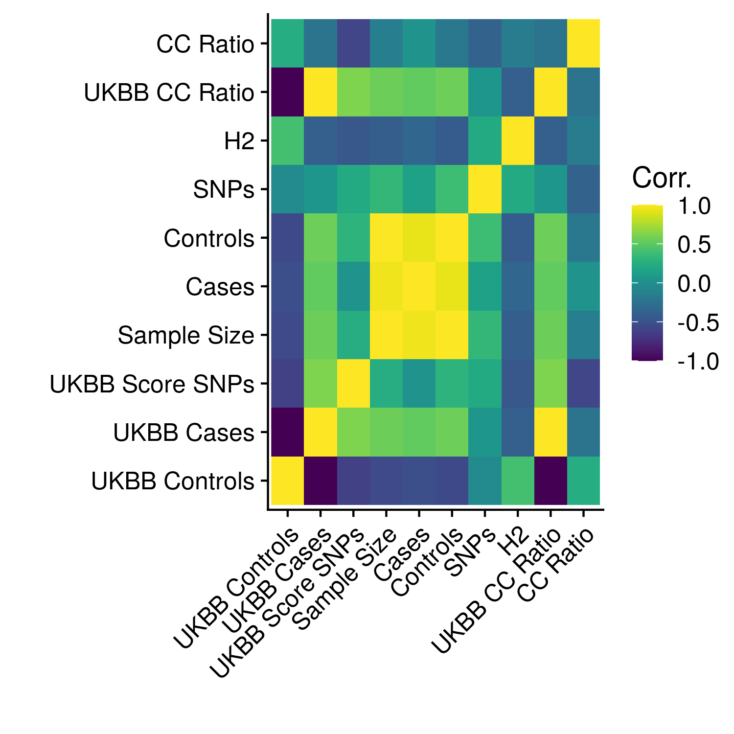
Figure 12.1: Heatmap of correlations between meta-statistics

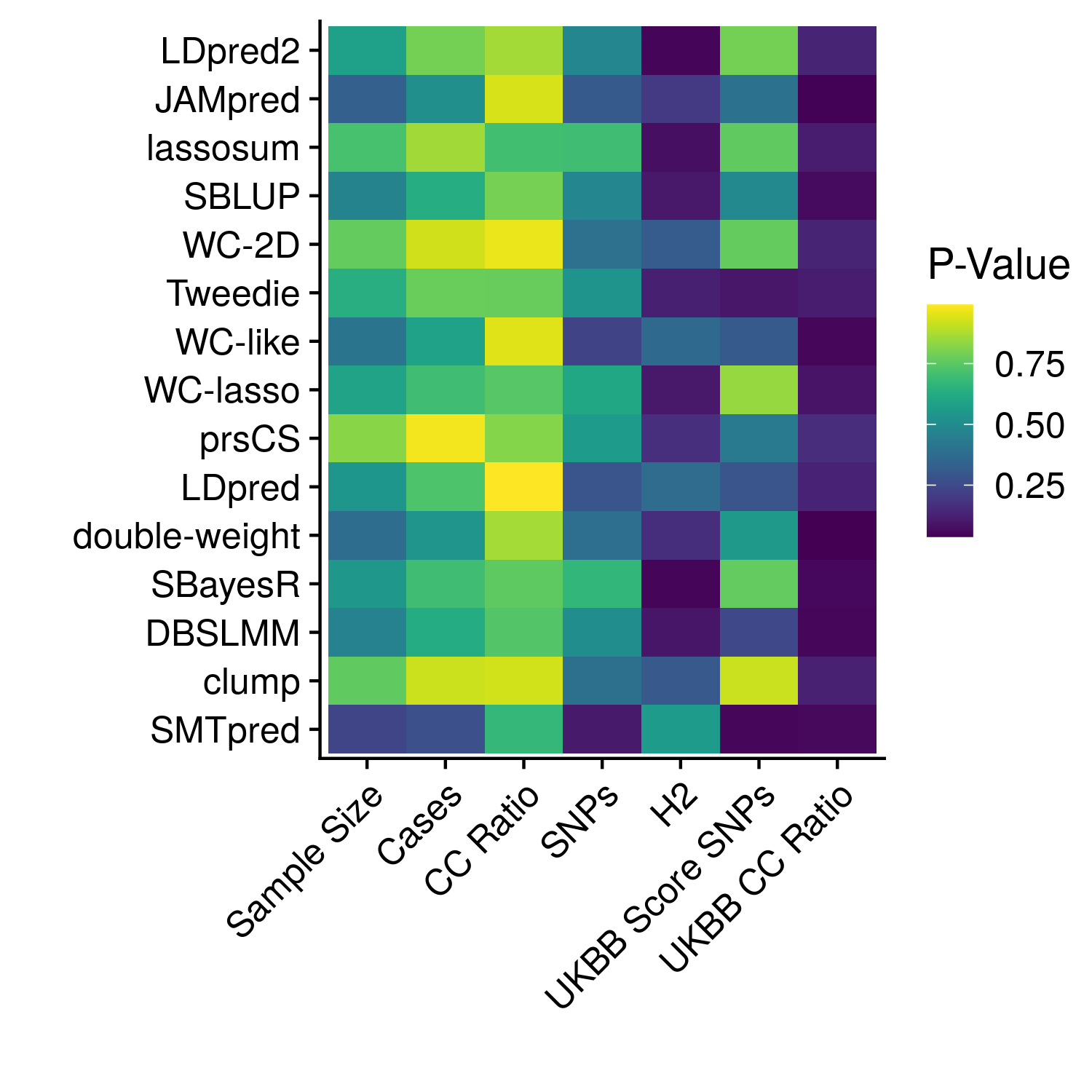
Figure 12.2: The significance of each meta-stat on the AUCs of each phenotype

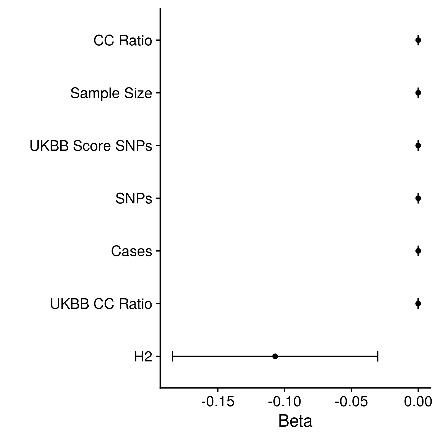
Figure 12.3: The effect of each meta-statistics on the AUCs of the best methods

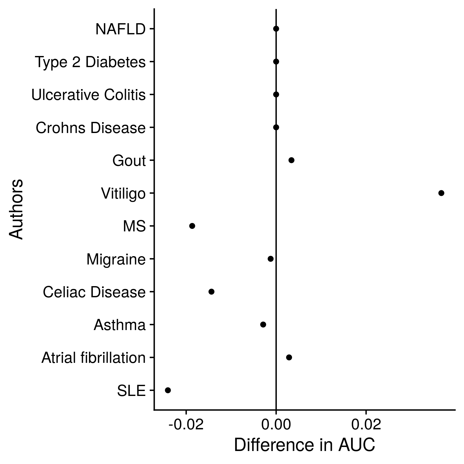
Figure 12.4: Comparison of training and testing AUCs

And the code is:

library(reshape2)
library(ggplot2)
library(cowplot)
library(stringr)
library(viridis)
theme_set(theme_cowplot())


#just need to add method_holder

method_dict <- read.table("local_info/method_names", stringsAsFactors = F)
author_dict <- read.table("local_info/disease_names", stringsAsFactors = F, sep = '\t')

convert_names <- function(x, the_dict = author_dict){
  y <- rep(NA, length(x))
  for(i in 1:length(x)){
    if(x[i] %in% the_dict[,1]){
      y[i] <- the_dict[the_dict[,1] == x[i], 2]
    }
  }
  return(y)
}


#1 - authors
#2 - the stats for best methods for each authors (setup data)
#3 - the stats for the single best methods for each authors (setup data)

meta_results <- readRDS("nonpred_results/meta_results.RDS")

#1 - authors
#2 - methods_auc - all aucs for all diseases and best methods
#3 - best_auc - all aucs for all disease and abs best
#4 - method_coef - regression coefs stratified by best methods
#5 - abs_coef - regression coefs between abs best
#6 - all_coef - regression coefs between all coefs
#7 - method_holder - count the number of times a method appears in the top
#8 - ttcomp

methods_setup <- meta_results[[2]] #nothing to do unless want to plot the AUC vs the meta-stat for each method or author
best_setup <- meta_results[[3]] #can plot the AUC vs meta-stats

temp <- meta_results[["method_auc"]]
temp <- temp[!duplicated(temp$author),]
temp <- temp[,c(6, 12:21, 23)]
temp[,1] <- convert_names(tolower(temp$author), author_dict)
temp <- temp[,-which(colnames(temp) == c("cases", "controls"))]
for(i in 2:ncol(temp)){
  temp[,i] <- signif(temp[,i], 3)
}
write.table(temp, "supp_tables/meta_reg_input.txt", col.names = T, row.names = F, sep = "\t", quote = F)

df <- read.table("supp_tables/med_endpoint_2.txt", stringsAsFactors = F, header = T, sep = "\t", fill = T)
df[,1] <- convert_names(tolower(df$author), author_dict)
write.table(df, "supp_tables/med_endpoint_3.txt", row.names = F, col.names = T, quote = F, sep = "\t")

######################################################################
#                   METHOD REGRESSIONS                            @
######################################################################

reg_coefs <- meta_results[[4]] #list elements is by methods, rows in the element is meta-stat
#c("sampe_size", "cases", "cases/controls", "snps", "h2", "uk_snps", "uk_case/uk_control", "uk_case")



stat_names <- c("uk_snps", "uk_beta_pdiff", "uk_len_pdiff", "sig6_gwas_snps", "sig8_gwas_snps", "len_pdiff",
                "effect_pdiff", "sampe_size", "ancestry", "snps", "h2", "uk_cc_ratio", "gwas_cc_ratio")
plot_stat_names <- c("PRS SNPs", "PRS Dist. by Effect", "PRS Dist. by Length", "GWAS SNPs < 1e-6", "GWAS SNPs < 1e-8",
                     "GWAS Dist. by Length", "GWAS Dist. by Effect", "GWAS Sample Size", "GWAS Ancestry", "GWAS SNPs",
                     "GWAS Heritability", "UKBB CC Ratio", "GWAS CC Ratio")


plot_df <- data.frame(matrix(0, nrow = length(reg_coefs), ncol = 4))
colnames(plot_df) <- c("method", "coef", "se", "p")
poss_methods <- convert_names(unique(methods_setup$method), method_dict)

all_plot_df <- list()
for(stat_ind in 1:length(stat_names)){
  for(i in 1:nrow(plot_df)){
    plot_df[i,1] <- poss_methods[i]
    plot_df[i,2:4] <- reg_coefs[[i]][stat_ind,c(1:2, 4)]
  }
  
  plot_df$method <- factor(plot_df$method, levels = plot_df$method[order(plot_df$coef)])
  
  the_plot <- ggplot(plot_df, aes(coef, method)) + geom_point() +
    geom_errorbar(aes(xmin = coef - se, xmax = coef + se, width = 0)) +
    geom_vline(xintercept = 0) +
    labs(x = "Regression Coefficient", y = "", caption = plot_stat_names[stat_ind]) 
    
  plot(the_plot)
  ggsave(paste0("reg_plots/reg_coef.", tolower(gsub("/", "", gsub(" ",  "_", stat_names)))[stat_ind], ".png"),
         the_plot + theme(plot.margin=unit(c(1,1,1,1), "cm")), height = 6, width = 6)
 
  plot_df$stat_name <- plot_stat_names[stat_ind]
  all_plot_df[[stat_ind]] <- plot_df 
}

plot_df <- do.call("rbind", all_plot_df)
the_plot <- ggplot(plot_df, aes(coef, method)) + geom_point() +
  facet_grid(cols = vars(stat_name), scales = "free") +
  geom_vline(xintercept = 0) +
  labs(x = "Regression Coefficient", y = "") +
  theme(strip.text.x = element_text(size = 8)) +
  scale_x_continuous(breaks = scales::pretty_breaks(n = 2))
plot(the_plot)
ggsave(paste0("reg_plots/reg_coef.facet.png"), the_plot, height = 6, width = 16)

plot_df[plot_df$p < 0.05,]


mat_beta <- matrix(0, nrow = length(reg_coefs), ncol = length(stat_names))
mat_pval <- matrix(0, nrow = length(reg_coefs), ncol = length(stat_names))
for(i in 1:length(reg_coefs)){
  for(j in 1:length(stat_names)){
    mat_beta[i,j] <- signif(reg_coefs[[i]][j,1], 3)
    mat_pval[i,j] <- signif(reg_coefs[[i]][j,4], 3)
  }
}
mat_beta <- cbind(poss_methods, data.frame(mat_beta))
mat_pval <- cbind(poss_methods, data.frame(mat_pval))
colnames(mat_beta) <- c("Method", plot_stat_names)
colnames(mat_pval) <- c("Method", plot_stat_names)
write.table(mat_beta, "supp_tables/meta_method.beta.txt", row.names = F, col.names = T, sep = "\t", quote = F)
write.table(mat_pval, "supp_tables/meta_method.pval.txt", row.names = F, col.names = T, sep = "\t", quote = F)

write.table(t(mat_beta)[,c(1:8)], "supp_tables/meta_method.beta.1.txt", row.names = T, col.names = F, sep = "\t", quote = F)
write.table(t(mat_beta)[,c(1,9:15)], "supp_tables/meta_method.beta.2.txt", row.names = T, col.names = F, sep = "\t", quote = F)
write.table(t(mat_pval)[,c(1:8)], "supp_tables/meta_method.pval.1.txt", row.names = T, col.names = F, sep = "\t", quote = F)
write.table(t(mat_pval)[,c(1,9:15)], "supp_tables/meta_method.pval.txt.2.txt", row.names = T, col.names = F, sep = "\t", quote = F)


######################################################################
#                   ABS BEST REGRESSIONS                            @
######################################################################

reg_coefs <- data.frame(meta_results[[5]])
colnames(reg_coefs) <- c("coef", "se", "z", "p")
reg_coefs$stat_names <- plot_stat_names
reg_coefs$stat_names <- factor(reg_coefs$stat_names, levels = reg_coefs$stat_names[order(reg_coefs$coef)])
reg_coefs <- reg_coefs[abs(reg_coefs$coef) < 5, ]

the_plot <- ggplot(reg_coefs, aes(coef, stat_names)) + geom_point() +
  geom_errorbar(aes(xmin = coef - se, xmax = coef + se, width = 0)) +
  geom_vline(xintercept = 0) +
  labs(x = "Regression Coefficient", y = "", caption = "Among Best Scores")
plot(the_plot)
ggsave(paste0("reg_plots/reg_coef.best.png"), the_plot, height = 6, width = 7)

for_table <- reg_coefs[,c(5,1,2,4)]
for_table[,2] <- signif(reg_coefs[,2], 3)
for_table[,3] <- signif(reg_coefs[,3], 3)
for_table[,4] <- signif(reg_coefs[,4], 3)
write.table(for_table, "supp_tables/meta_reg.disease.txt", row.names = F, col.names = T, sep = "\t", quote = F)

#to double check
df <- meta_results[["method_auc"]]
best_names <- readRDS("nonpred_results/best_names.RDS")
df <- df[df$name %in% best_names,]

######################################################################
#                   ALL AUC REGRESSIONS                            @
######################################################################

reg_coefs <- data.frame(meta_results[[6]])
colnames(reg_coefs) <- c("coef", "se", "z", "p")
reg_coefs$stat_names <- plot_stat_names
reg_coefs$stat_names <- factor(reg_coefs$stat_names, levels = reg_coefs$stat_names[order(reg_coefs$coef)])
reg_coefs <- reg_coefs[abs(reg_coefs$coef) < 5, ]

the_plot <- ggplot(reg_coefs, aes(coef, stat_names)) + geom_point() +
  geom_errorbar(aes(xmin = coef - se, xmax = coef + se, width = 0)) +
  geom_vline(xintercept = 0) +
  labs(x = "Regression Coefficient", y = "", caption = "Among All Scores")
plot(the_plot)
ggsave(paste0("reg_plots/reg_coef.all.png"), the_plot, height = 6, width = 7)

for_table <- reg_coefs[,c(5,1,2,4)]
for_table[,2] <- signif(reg_coefs[,2], 3)
for_table[,3] <- signif(reg_coefs[,3], 3)
for_table[,4] <- signif(reg_coefs[,4], 3)
write.table(for_table, "supp_tables/meta_reg.all.txt", row.names = F, col.names = T, sep = "\t", quote = F)


######################################################################
#                   METHODS BEST AT EXTREMES                            @
######################################################################
exit()
method_ex <- data.frame(meta_results[[7]])
method_ex$stat <- paste(rep(plot_stat_names[plot_stat_names != "GWAS Ancestry"], each = 2), c("", "Rev."))
method_ex  <- melt(method_ex, id.vars = "stat")
method_ex$variable <- convert_names(method_ex$variable, method_dict)

the_plot <- ggplot(method_ex, aes(variable, stat, fill = value)) + geom_raster() +
  scale_fill_viridis() +
  theme(axis.text.x = element_text(angle = 45, vjust = 1, hjust=1)) +
  labs(x = "", y = "", fill = "Times In\nTop 10")
plot(the_plot)
ggsave(paste0("reg_plots/method_extreme.png"), the_plot, height = 7, width = 7)

method_ex <- method_ex[grepl("GWAS", method_ex$stat),]
method_ex$stat <- unlist(lapply(strsplit(method_ex$stat, "GWAS"), function(x) x[2]))
method_ex$stat <- trimws(method_ex$stat)
method_ex$stat[grepl("SNP", method_ex$stat)] <- paste0("No. ", method_ex$stat[grepl("SNP", method_ex$stat)])
the_plot <- ggplot(method_ex, aes(variable, stat, fill = value)) + geom_raster() +
  scale_fill_viridis() +
  theme(axis.text.x = element_text(angle = 45, vjust = 1, hjust=1)) +
  labs(x = "", y = "", fill = "Times In\nTop 10")
plot(the_plot)
ggsave(paste0("reg_plots/method_extreme_gwas.png"), the_plot, height = 5, width = 7)

to_save <-  data.frame(meta_results[[7]])
to_save$stat <- paste(rep(plot_stat_names[plot_stat_names != "GWAS Ancestry"], each = 2), c("", "Rev."))
colnames(to_save) <- convert_names(colnames(to_save), method_dict)
to_save <- to_save[,c(ncol(to_save), 1:(ncol(to_save)-1))]
write.table(to_save[,c(1,2:7)], "supp_tables/method_extreme.1.txt", row.names = F, col.names = T, quote = F, sep = "\t")
write.table(to_save[,c(1,8:16)], "supp_tables/method_extreme.2.txt", row.names = F, col.names = T, quote = F, sep = "\t")
write.table(to_save[,c(1,11:16)], "supp_tables/method_extreme.3.txt", row.names = F, col.names = T, quote = F, sep = "\t")

######################################################################
#                  TRAIN/TEST                          @
######################################################################

tt_df <- data.frame(meta_results[[8]])
colnames(tt_df) <- c("diff_conc", "diff_survfit", "diff_auc", "diff_or")
tt_df$disease <- convert_names(meta_results[[1]])

mean(tt_df$diff_auc)
sd(tt_df$diff_auc)/sqrt(nrow(tt_df))

melt_tt <- melt(tt_df, id.vars = "disease")
melt_tt$variable <- convert_names(melt_tt$variable, cbind(colnames(tt_df)[1:4], c("Conc.", "Hazard", "AUC", "OR")))

the_plot <- ggplot(melt_tt, aes(x = value, y = disease, )) + geom_point() + 
  facet_grid(cols = vars(variable), scales = "free") +
  geom_vline(xintercept = 0) +
  scale_x_continuous(breaks = scales::pretty_breaks(n = 3)) +
  labs(x = "Statistic Difference")
plot(the_plot)
ggsave(paste0("reg_plots/reg_coef.tt.png"), the_plot, height = 6, width = 12)

tt_df <- data.frame(meta_results[[8]])
colnames(tt_df) <- c("diff_conc", "diff_survfit", "diff_auc", "diff_or")
tt_df$disease <- convert_names(meta_results[[1]])
tt_df <- tt_df[,c(5,1,2,3,4)]
tt_df[,2] <- signif(tt_df[,2], 3)
tt_df[,3] <- signif(tt_df[,3], 3)
tt_df[,4] <- signif(tt_df[,4], 3)
tt_df[,5] <- signif(tt_df[,5], 3)
write.table(tt_df, "supp_tables/train-test.txt", row.names = F, col.names = T, sep = "\t", quote = F)