4 Getting the Summary Statistics

Now we have to get the actual summary statistics. A key consideration is to pull from summary statistics with the largest possibly underlying sample size, because it will produce the most accurate estimates. The studies can be obtained with:

#Files that are already haromized

mkdir Bentham
wget -O Bentham/raw_bentham.ss.gz ftp://ftp.ebi.ac.uk/pub/databases/gwas/summary_statistics/BenthamJ_26502338_GCST003156/harmonised/26502338-GCST003156-EFO_0002690-build37.f.tsv.gz

mkdir Christophersen
wget -O Christophersen/raw_christophersen.ss.gz ftp://ftp.ebi.ac.uk/pub/databases/gwas/summary_statistics/ChristophersenIE_28416818_GCST004296/harmonised/28416818-GCST004296-EFO_0000275-build37.f.tsv.gz

mkdir Demenais
wget -O Demenais/raw_demenais.ss.gz ftp://ftp.ebi.ac.uk/pub/databases/gwas/summary_statistics/DemenaisF_29273806_GCST005212/harmonised/29273806-GCST005212-EFO_0000270-build37.f.tsv.gz

mkdir Dubois
wget -O Dubois/raw_dubois.ss.gz ftp://ftp.ebi.ac.uk/pub/databases/gwas/summary_statistics/DuboisPC_20190752_GCST000612/harmonised/20190752-GCST000612-EFO_0001060-Build37.f.tsv.gz

mkdir Liu-1
wget -O Liu-1/raw_liu-1.ss.gz ftp://ftp.ebi.ac.uk/pub/databases/gwas/summary_statistics/LiuJZ_26192919_GCST003044/harmonised/26192919-GCST003044-EFO_0000384-Build37.f.tsv.gz

mkdir Liu-2
wget -O Liu-2/raw_liu-2.ss.gz ftp://ftp.ebi.ac.uk/pub/databases/gwas/summary_statistics/LiuJZ_26192919_GCST003045/harmonised/26192919-GCST003045-EFO_0000729-Build37.f.tsv.gz

mkdir Malik
wget -O Malik/raw_malik.ss.gz ftp://ftp.ebi.ac.uk/pub/databases/gwas/summary_statistics/MalikR_29531354_GCST005838/harmonised/29531354-GCST005838-EFO_0000712-build37.f.tsv.gz

mkdir Michailidou
wget -O Michailidou/raw_michailidou.ss.gz ftp://ftp.ebi.ac.uk/pub/databases/gwas/summary_statistics/MichailidouK_29059683_GCST004988/harmonised/29059683-GCST004988-EFO_0000305-build37.f.tsv.gz

mkdir Nikpay
wget -O Nikpay/raw_nikpay.ss.gz ftp://ftp.ebi.ac.uk/pub/databases/gwas/summary_statistics/NikpayM_26343387_GCST003116/harmonised/26343387-GCST003116-EFO_0000378-build37.f.tsv.gz

mkdir Okada
wget -O Okada/raw_okada.ss.gz ftp://ftp.ebi.ac.uk/pub/databases/gwas/summary_statistics/OkadaY_24390342_GCST002318/harmonised/24390342-GCST002318-EFO_0000685-Build37.f.tsv.gz

mkdir Onengut
wget -O Onengut/raw_onengut.ss.gz ftp://ftp.ebi.ac.uk/pub/databases/gwas/summary_statistics/Onengut-GumuscuS_25751624_GCST005536/harmonised/25751624-GCST005536-EFO_0001359-Build37.f.tsv.gz

mkdir Phelan
wget -O Phelan/raw_phelan.ss.gz ftp://ftp.ebi.ac.uk/pub/databases/gwas/summary_statistics/PhelanCM_28346442_GCST004462/harmonised/28346442-GCST004462-EFO_0001075-Build37.f.tsv.gz

mkdir Schumacher
wget -O Schumacher/raw_schumacher.ss.gz ftp://ftp.ebi.ac.uk/pub/databases/gwas/summary_statistics/SchumacherFR_29892016_GCST006085/harmonised/29892016-GCST006085-EFO_0001663-build37.f.tsv.gz

mkdir Tsoi
wget -O Tsoi/raw_tsoi.ss.gz ftp://ftp.ebi.ac.uk/pub/databases/gwas/summary_statistics/TsoiLC_23143594_GCST005527/harmonised/23143594-GCST005527-EFO_0000676-Build37.f.tsv.gz

mkdir Rheenen
wget -O Rheenen/raw_rheenen.ss.gz ftp://ftp.ebi.ac.uk/pub/databases/gwas/summary_statistics/vanRheenenW_27455348_GCST004692/harmonised/27455348-GCST004692-EFO_0000253-build37.f.tsv.gz


#Files that need to be harmonized

mkdir Jin
wget -O Jin/ ftp://ftp.ebi.ac.uk/pub/databases/gwas/summary_statistics/JinY_30674883_GCST007111/JinY_PrePMID_GWAS123chr*

mkdir Namjou
wget -O Namjou/raw_namjou.ss ftp://ftp.ebi.ac.uk/pub/databases/gwas/summary_statistics/NamjouB_31311600_GCST008468/NamjouB_31311600_NAFLD.txt

mkdir Lopez
wget -O Lopez/raw_lopez.ss ftp://ftp.ebi.ac.uk/pub/databases/gwas/summary_statistics/Lopez-IsacE_31672989_GCST009131/Lopez-Isac_prePMID_META_GWAS_SSc.meta.txt

mkdir Xie
wget -O Xie/raw_xie.ss.gz ftp://ftp.ebi.ac.uk/pub/databases/gwas/summary_statistics/XieJ_32231244_GCST010004/Trans-ethnic_GWAS_meta-analysis_without_replication.txt.gz

mkdir Mahajan
wget -O Mahajan/raw_mahajan.ss ftp://ftp.ebi.ac.uk/pub/databases/gwas/summary_statistics/MahajanA_29632382_GCST007515/T2D_TranEthnic.BMIunadjusted.txt

mkdir Shah
wget -O Shah/raw_shah.ss.gz ftp://ftp.ebi.ac.uk/pub/databases/gwas/summary_statistics/ShahS_31919418_GCST009541/ShahS_31919418_HeartFailure.gz

mkdir Kottgen
wget -O Kottgen/raw_kottgen.ss.gz ftp://ftp.ebi.ac.uk/pub/databases/gwas/ftp://ftp.ebi.ac.uk/pub/databases/gwas/summary_statistics/KottgenA_23263486_GCST001790/GUGC_MetaAnalysis_Results_Gout.csv.zip

#Note there is also data from 23andMe that needs to be processed

This is basically just a series of wget’s to the FTP server of the GWAS catalog. I am also using some files from 23andMe, however these cannot be openly downloaded on GWAS Catalog.

Lastly, a committee member of mine asked me to look into a few pyschiatric related traits, which has summary statistics available on request or within the pyschiatric genomics consortium (https://www.med.unc.edu/pgc/download-results/). While I likely could have followed a similar request approach to recieve a few more sets, the total number of 25 seems like a good stopping point.

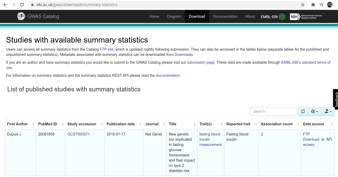
Figure 4.1: test

If you want to manually download just one summary statistic, or you want a more pictoral description of the summary statistics then you can access https://www.ebi.ac.uk/gwas/downloads/summary-statistics . There are other GWAS results that are not fully summary statistics, as the motivation of this project is to assess different methods we want the full summary statistics for many SNPs, not just the signifiant ones. Plus, from the full summary statistics we can always reduce down to only a significant-only score.

4.1 Prepare Variants

As we’ve already QCd the individuals, the other half of the QC is on the variants. That can be easily done by keeping variants that have an imputation INFO score above 0.9, and removing duplicate variants (or variants that are tri-allelic). The INFO score refers to the probability the imputation software has in calling the allele the way it did, we only want high probability variants. We do not want duplicate variants because its tri-allele option slightly increases the probability that it was called or otherwise referred to incorrectly at some point in its analysis. Moreover, the biology is likely more complicating (perhaps not agreeing with the assumptions of the downstream methods), and sorting gets easier.

The other variant level of QC nescessary is on the minor allele frequency and hardy weinberg equilibrium, but we can do that after the white, british group has already be determined. Note that in other analyses this step could be done now, but with file formats as I have (bgen now, plink later), I will wait for this step.

The script used to pull this off is as follows, where the ukb_mfi_all.txt file originates from the UKBB directly.

#Reduce the full list of RSIDs to those with INFO score greater than 0.9
cat ~/athena/ukbiobank/qc/imputed/ukb_mfi_all.txt | awk '$8 > 0.9 {print $0}' > common_files/impute_rsids

#Extract all of the duplicated RSIDs
cat ~/athena/ukbiobank/qc/imputed/ukb_mfi_all.txt | cut -f2 | sort | uniq -d > common_files/dup_ids

#Remove the duplicated RSIDs from the full list of (INFO approved) SNPs
cat common_files/impute_rsids | fgrep -w -v -f common_files/dup_ids > common_files/temp

mv common_files/temp common_files/impute_rsids

4.2 Standardize the Summary Statistics

This is a big step. The underlying motivation is that all of the files need to look the same so downstream coding is far easier. In this process we will convert the base pair positions, or the genome build, so they match the UK Biobank. The can simply be done by matching the rsIDs. We will also remove ambigious SNPs, and then flip the remaining SNPs so they match the UK Biobank strand. The exact procedures, and a few other small changes are described in the script.

library(vroom)
library(stringr)
library(bigsnpr)

options(warn=2)

#impute <- as.data.frame(vroom("common_files/impute_rsids", col_names = F))
impute <- read.table("common_files/impute_rsids", header = F, stringsAsFactors = F)
colnames(impute) <- c("LOC", "SNP", "POS", "A1", "A2", "MAF", "AX", "INFO")

#First remove SNPs where the base is longer than one allele
#And make sure the SNP is either A, C, G, T
#Remove ambigous SNPs, those where the bases are actually pairs
impute <- impute[nchar(impute$A1) == 1 & nchar(impute$A2) == 1,]
impute <- impute[impute$A1 %in% c("A", "C", "G", "T") & impute$A2 %in% c("A", "C", "G", "T"),]
impute <- impute[!((impute$A1 == "A" & impute$A2 == "T") |
             (impute$A1 == "T" & impute$A2 == "A") |
             (impute$A1 == "G" & impute$A2 == "C") |
             (impute$A1 == "C" & impute$A2 == "G")),]


adjust_ss <- function(author){

  #Start by reading in the summary statistics file and a parameters file that states the column
  #names of the desired columns
  #ss <- as.data.frame(vroom(paste0(author, "/raw_", tolower(author), ".ss.gz")))
  ss <- read.table(paste0(author, "/raw_", tolower(author), ".ss.gz"), stringsAsFactors=F, header = T)
  params <- read.table(paste0(author, "/parameters"), stringsAsFactors=F)

  system(paste0("echo clean notes > ", author, "/clean.log"))
  system(paste0("echo after read: ", nrow(ss), " >> ", author, "/clean.log"))

  #Check if there are missing columns, and fill them in just so things don't go haywire below
  missing_cols <- params[!(params[,1] %in% colnames(ss)),1]
  if(length(missing_cols) > 0){
    if("NO_CHR" %in% missing_cols){
      ss$NO_CHR <- 0
    }
    if("NO_POS" %in% missing_cols){
      ss$NO_POS <- 0
    }
    if("NO_SE" %in% missing_cols){
      ss$NO_SE <- 0
    }
  }


  #Construct a common ss object, with common column names based on the manually curated params
  ss <-  ss[,c(which(colnames(ss) == params[1,1]),
               which(colnames(ss) == params[2,1]),
               which(colnames(ss) == params[3,1]),
               which(colnames(ss) == params[4,1]),
               which(colnames(ss) == params[5,1]),
               which(colnames(ss) == params[6,1]),
               which(colnames(ss) == params[7,1]),
               which(colnames(ss) == params[8,1]))]
  colnames(ss) <- c("CHR", "BP", "RSID", "A1", "A2", "SE", "BETA", "P")
  ss$A1 <- toupper(ss$A1)
  ss$A2 <- toupper(ss$A2)
  ss <- ss[!is.na(ss$RSID),]
  ss <- ss[!is.na(ss$BETA),]
  ss <- ss[!is.na(ss$P),]

  system(paste0("echo after remove NA: ", nrow(ss), " >> ", author, "/clean.log"))

  #Remove duplicate SNP IDs
  dup_ids <- ss$RSID[duplicated(ss$RSID)]
  ss <- ss[!(ss$RSID %in% dup_ids),]

  system(paste0("echo after remove duplicated IDs: ", nrow(ss), " >> ", author, "/clean.log"))

  #First remove SNPs where the base is longer than one allele
  #And make sure the SNP is either A, C, G, T
  #Remove ambigous SNPs, those where the bases are actually pairs
  ss <- ss[nchar(ss$A1) == 1 & nchar(ss$A2) == 1,]
  ss <- ss[ss$A1 %in% c("A", "C", "G", "T") & ss$A2 %in% c("A", "C", "G", "T"),]
  system(paste0("echo after remove non ACGT SNPs: ", nrow(ss), " >> ", author, "/clean.log"))

  ss <- ss[!((ss$A1 == "A" & ss$A2 == "T") |
             (ss$A1 == "T" & ss$A2 == "A") |
             (ss$A1 == "G" & ss$A2 == "C") |
             (ss$A1 == "C" & ss$A2 == "G")),]

  system(paste0("echo after remove ambigous SNPs: ", nrow(ss), " >> ", author, "/clean.log"))

  #Make sure the imputation reference and the ss objects have the same number of SNP IDs
  ss$RSID <- tolower(ss$RSID)
  ss <- ss[ss$RSID %in% impute$SNP,]
  sub_impute <- impute[impute$SNP %in% ss$RSID,]

  system(paste0("echo after remove SNPs not in the UKBB imputation: ", nrow(ss), " >> ", author, "/clean.log"))

  if(nrow(ss) != nrow(sub_impute)){
    print("SIZE MISMATCH")
  }

  #Extract the chromosomes from the imputation reference object
  #Sometimes the chromosome is not listed for an object
  #But since the rows seem to be ordered we can impute the chromosome based on the surrounding chromosomes
  chr <- sapply(strsplit(sub_impute[,1], ":"), function(x) x[[1]])
  for(i in as.character(1:22)){
    if(i %in% chr){
      min_ind <- min(which(chr==i))
      max_ind <- max(which(chr==i))
      chr[min_ind:max_ind] <- i
    }
  }

  #Finish cleaning up the chr, because "X" could be there instead of 23
  chr[!(chr %in% as.character(1:22))] <- "23"
  chr <- as.numeric(chr)

  #Sort the imputation reference and the ss objects so they are the same order
  #Then assign the imputation chr and pos to the ss object
  ss <- ss[order(ss$RSID)[rank(sub_impute$SNP)],]
  ss <- ss[order(chr, sub_impute$POS),]
  sub_impute <- sub_impute[order(chr, sub_impute$POS),]
  chr <- chr[order(chr)]

  #make the ss object chromosome and position the same as the imputed object
  ss$CHR <- chr
  ss$BP <- sub_impute$POS


  #If there is a name in the parameters that states CHANGE_BOTH assuming that it's not BETA but OR
  #This would just be a simple exponentiation
  if(nrow(params) > 8){
    if(params[9,1] == "CHANGE_BOTH"){
      #will assume that the effect name is for odds ratio
      #following the walds ratio tests can just switch things over assuming a normal distribution
      #This may not be exactly what was completed in the published GWAS, but it should be a good approximation
      #And few methods seem to use the SE column anyway
      ss$BETA <- log(ss$BETA)
      ss$SE <- abs(ss$BETA/qnorm(ss$P))
    }
  }


  #use the bignspr function to flip and reverse the summmary statistics
  colnames(ss) <- c("chr", "pos", "rsid", "a0", "a1", "beta_set", "beta", "p")
  save_impute_cols <- colnames(sub_impute)
  colnames(sub_impute) <- c("loc", "rsid", "pos", "a0", "a1", "maf", "ax", "info")
  sub_impute$chr <- ss$chr
  ss <- snp_match(ss, sub_impute)
  ss <- ss[,c(1,2,5,3,4,6,7,8)]
  colnames(ss) <- c("CHR", "BP", "RSID", "A1", "A2", "SE", "BETA", "P")
  colnames(sub_impute) <- save_impute_cols
  
  system(paste0("echo after removing SNPs that do not flip: ", nrow(ss), " >> ", author, "/clean.log"))


  #Finally add in effective sample size, as defined by PLINK
  notes <- read.table(paste0(author, "/notes"), sep = '\t', stringsAsFactors=F)
  ss$ESS <- round(4/(1/as.numeric(notes[4,1]) + 1/as.numeric(notes[5,1])))

  #According to LDPRED-2 it is a good idea to compare to a validation set following:
  sd_ss <- 2/(ss$SE * sqrt(ss$ESS))

  #For the validation set I will use summary statistics from the FinnGen Biobank
  #First I have to go through several steps to line everything up
  finn_notes <- read.table("../finngen_ss/sample_size", stringsAsFactors=F)
  if(author %in% finn_notes[,4]){
    finn_ess <- 4/((1/finn_notes[finn_notes[,4] == author,2]) + (1/finn_notes[finn_notes[,4] == author,3]))
    finn_pheno <- finn_notes[finn_notes[,4] == author,1]

    finn_ss <- read.table(paste0("../finngen_ss/summary_stats_finngen_r3_", finn_pheno, ".gz"), header =F, stringsAsFactors=F, sep = '\t')  
    finn_ss <- finn_ss[finn_ss[,5] %in% ss$RSID,]
    dup_rs <- finn_ss[duplicated(finn_ss[,5]), 5]
    finn_ss <- finn_ss[!finn_ss[,5] %in% dup_rs,]

    finn_rs <- finn_ss[,5]
    finn_sd <- finn_ss[,9]
  
    finn_sd <- c(finn_sd, rep(0, (nrow(ss) - length(finn_rs))))
    finn_rs <- c(finn_rs, ss$RSID[!(ss$RSID %in% finn_rs)])
    finn_sd <- finn_sd[order(finn_rs)[rank(ss$RSID)]]

    finn_sd <- 2/(finn_sd * sqrt(finn_ess))

    good_rs <- ss$RSID[sd_ss < 2 * finn_sd & sd_ss > 0.5 * finn_sd]
    good_rs <- c(good_rs, ss$RSID[finn_sd == Inf])
    ss <- ss[ss$RSID %in% good_rs,]
  }
  system(paste0("echo after removing SNPs that do not align with FinnGen: ", nrow(ss), " >> ", author, "/clean.log"))


  #Now write the answer
  write.table(ss, paste0(author, "/clean_", tolower(author), ".txt"), row.names = F, col.names = T, sep = '\t', quote = F)
  system(paste0("gzip ", author, "/clean_", tolower(author), ".txt"))
}


all_authors <- read.table("common_files/list_authors", stringsAsFactors=F)
for(author in all_authors[,1]){
  print(author)
  adjust_ss(author)
}

As you can see at the bottom of the script I am looping over all of the sets of summary statistics, which are organized so each set belongs to its own directory with the name raw_author.ss.gz. Also within the directory are two files, “notes” and “parameters”. The notes files contains some meta-information and the parameters names the column names referring to a different statistic or type of information. Specifically “notes” contains with each new line: author name, disease name, total sample size, case sample size, control sample size, ancestry of GWAS and title of originating publication. Specifically “parameters” contains the chromosome, base pair location, rs prefixed variant ID, effect allele (or first allele), non-effect allele (or second allele), standard error of the effect, effect, and p value. There is an optional ninth line with the term CHANGE_BOTH which indicates the effect is an odds ratio and needs to be converted to a beta values (spanning from negative to positive).

With the script read in for reference, I want to clearly list everything that I am kicking out of the summary statistics. To do this I will call examples from the Phelan summary statistics. The raw download appears as:

ss <- read.table("../raw_ss/Phelan/raw_phelan.ss.gz", stringsAsFactors=F, header=T, nrows = 10)
head(ss)

##          rsid Chromosome Position Effect               Baseline     EAF
## 1 rs145072688          1    10352     TA                      T 0.42360
## 2 rs376342519          1    10616      C CCGCCGTTGCAAAGGCGCGCCG 0.99100
## 3 rs201725126          1    13116      G                      T 0.17040
## 4 rs200579949          1    13118      G                      A 0.17040
## 5  rs75454623          1    14930      G                      A 0.52060
## 6 rs199856693          1    14933      A                      G 0.04797
##   R2_oncoarray overall_OR overall_SE overall_chi2 overall_pvalue
## 1       0.4713  -0.019590    0.02150      0.83020         0.3622
## 2       0.8243   0.013190    0.09657      0.01867         0.8913
## 3       0.3866   0.006643    0.02865      0.05375         0.8167
## 4       0.3866   0.006643    0.02865      0.05375         0.8167
## 5       0.4054   0.022960    0.02127      1.16500         0.2804
## 6       0.3547   0.070590    0.06168      1.31000         0.2524

INFO Score < 0.9 - only want alleles whose identity are certain
Non-duplicate - want simple base subsititions that are easier to call and process

ss <- read.table("../raw_ss/Phelan/raw_phelan.ss.gz", stringsAsFactors=F, header=F, skip = 629730, nrows = 2)
print(ss)

##          V1 V2        V3 V4 V5     V6     V7        V8      V9    V10      V11
## 1 rs7517916  1 109370390  A  C 0.2888 0.7717 -0.046220 0.01603 8.3130 0.003937
## 2 rs7517916  1 109370390  G  C 0.3199 0.8600  0.009952 0.01498 0.4416 0.506400

We can see the SNP rs7517916 is tri-allelic, with alleles A, C, G. As this tri-system makes calling more difficult, and strand determination near impossible we discard this SNP altogether.

ACGT - similar to above, limiting to the most simple cases of base pair subtitition or single nucleotide polymorphism

ss <- read.table("../raw_ss/Phelan/raw_phelan.ss.gz", stringsAsFactors=F, header=F, skip = 1, nrows = 2)
print(ss)

##            V1 V2    V3 V4                     V5     V6     V7       V8      V9
## 1 rs145072688  1 10352 TA                      T 0.4236 0.4713 -0.01959 0.02150
## 2 rs376342519  1 10616  C CCGCCGTTGCAAAGGCGCGCCG 0.9910 0.8243  0.01319 0.09657
##       V10    V11
## 1 0.83020 0.3622
## 2 0.01867 0.8913

Here we have two clear examples of SNPs whose alleles are not just A, C, G, T. This paradigm does not work with our strand flipping capabilities (and is harder to call by most sequencing technologies) so we again discard these types of SNPs.

Non-ambigous - If the alleles are A and T or C and G, these are called ambigous and will present a problem later on when we try to determine if the standedness of the summary statistics match the strand of our data. This is likely possibly to figure out through allele frequencies, but again, it’s not worth the risk

ss <- read.table("../raw_ss/Phelan/raw_phelan.ss.gz", stringsAsFactors=F, header=F, skip = 9, nrows = 1)
print(ss)

##            V1 V2    V3   V4 V5     V6    V7      V8      V9     V10    V11
## 1 rs201931625  1 15274 TRUE  A 0.6996 0.432 0.00715 0.02451 0.08508 0.7705

The two alleles described are T and A. As stated, since flipping these alleles leaves us where we started we must again discard this SNP since flipping is impossible.

Non-X chromosome - As chromosome 23 is very different between men and women (and it’s relatively short), we would likely have to do some special case regressions to set up an accurate model, which makes it easiest just to forget it. Note, no example in Phelan but if it did exist the chromosome column would be X, Y or 23.
Non-reversable SNPs - We need to flip (or reverse) SNPs such that the allele identities of the summary statistics match the allele identities of the genotypes. We do this by assuming that if they do not line up then we can swap A with T, or C with G (and the converse), and things will work. However, if just one of the SNPs matches after reversing then we have a weird problem that is easiest to resolve by removing the troublesome SNP.

sst <- read.table("../raw_ss/Phelan/raw_phelan.ss.gz", stringsAsFactors=F, header=F, skip = 280, nrows = 1)
ref <- read.table("../raw_ss/common_files/impute_rsids", stringsAsFactors=F, header=F, skip = 5995727, nrow = 1)
print(sst)

##           V1 V2     V3   V4 V5      V6    V7      V8      V9     V10   V11
## 1 rs12184267  1 715265 TRUE  C 0.04354 0.371 0.01388 0.05711 0.05906 0.808

print(ref)

##             V1         V2     V3 V4   V5        V6   V7       V8
## 1 1:715265_C_T rs12184267 715265  C TRUE 0.0366377 TRUE 0.926915

This is an example of reversed SNPs, the A1 of the summary statistic does not match the A1 of the reference data. Therefore we swap the position of the alleles in the summary statistics and similarly reverse the beta or effect value.

sst <- read.table("../raw_ss/Phelan/raw_phelan.ss.gz", stringsAsFactors=F, header=F, skip = 375350, nrows = 1)
ref <- read.table("../raw_ss/common_files/impute_rsids", stringsAsFactors=F, header=F, skip = 6358575, nrow = 1)
print(sst)

##          V1 V2       V3   V4 V5       V6  V7     V8    V9    V10    V11
## 1 rs1390473  1 64804379 TRUE  C 0.001289 -99 0.4462 1.128 0.1566 0.6923

print(ref)

##               V1        V2       V3 V4 V5         V6 V7       V8
## 1 1:64804379_A_G rs1390473 64804379  A  G 0.00451314  A 0.934127

This is an example of a SNP that needs to be flipped since the summary statistic is on one strand while the complementary base pairs are described in the reference data. In this case the beta or effect value stays the same because the same information is being described in both the summary statistic and reference data, just not using the same language or strand.

sst <- read.table("../raw_ss/Phelan/raw_phelan.ss.gz", stringsAsFactors=F, header=F, skip = 15414049, nrows = 1)
ref <- read.table("../raw_ss/common_files/impute_rsids", stringsAsFactors=F, header=F, skip = 7679970, nrow = 1)
print(sst)

##          V1 V2       V3   V4 V5       V6     V7     V8   V9    V10    V11
## 1 rs8120968 20 61831053 TRUE  G 4.62e-05 0.5318 0.8177 1.37 0.3563 0.5506

print(ref)

##                V1        V2       V3 V4 V5         V6 V7       V8
## 1 20:61831053_G_A rs8120968 61831053  G  A 0.00120068  A 0.926685

This is an example of a SNP that is not resolved after either flipping or reversing. In short, the G allele appears to be on the reference stand but the T allele does not. With this confusion we decide to play it safe and discard the SNP altogether.

Standard error outliers - Following the supplementary of the method LDPRED2, we can compare standard errors between studies to determine if SNPs are outliers in their effects. For this task I have pulled results from FinnGen Biobank, which while not matching ancestry well with British, does a decent enough job of falling within the European category to work.

The remaining steps mostly involve re-aligning, changing column names and the like. Note that we take such a liberal stance on removing SNPs because we assume there is a density of summary statistics such that the removal of any SNP will still leave behind another SNP within a given causal locus that is ultimately important for prediction.

4.3 Heritability Estimation

Many downstream methods require heritability estimates of the trait using the corresponding summary statistics. While many, many heritability estimate methods exist I am limited to those that only require summary statistics, of which I know of 2: Linkage Disequilibirum Score Regression and High-Definition Likelihood (HDL). The first step required is to munge the summary statistics, or further QC them following a munge_sumstats script provided by LDSC. The script for which is simple:

cat common_files/list_authors | while read author;do
  low_author=`echo "$author" | tr '[:upper:]' '[:lower:]'`
  munge_sumstats --sumstats ${author}/clean_${low_author}.txt.gz --N-col ESS --out ${author}/${low_author}.munged
done

The next step is the actual heritability estimation, which luckily only requires a simple command line call for each method. We do have to be careful however in making sure all of the columns match up in the arguments. The script therefore looks like:

cat common_files/list_authors | while read author;do
#author=Tsoi
  low_author=`echo "$author" | tr '[:upper:]' '[:lower:]'`
  ldsc --h2 ${author}/${low_author}.munged.sumstats.gz --ref-ld-chr ~/athena/refs/eur_w_ld_chr/ --w-ld-chr ~/athena/refs/eur_w_ld_chr/ --out ${author}/${low_author}.h2

  Rscript ~/Programs/HDL/HDL.run.R \
    gwas.df=${author}/${low_author}.munged.sumstats.gz \
    LD.path=~/athena/refs/UKB_imputed_SVD_eigen99_extraction \
    output.file=${author}/${low_author}.HDL.h2.Rout
done

We can compile all of the heritability estimates, which are currently sitting in log files, into a single file using a simple bash script. Additionaly, we can include other useful information that may be needed downstream, such as sample size and number of SNPs. The script looks like:



echo author,trait,sampe_size,cases,controls,ancestry,snps,ldsc_h2,ldsc_h2_se,hdl_h2,hdl_h2se > meta_stats

cat common_files/list_authors | while read author;do
  low_author=`echo "$author" | tr '[:upper:]' '[:lower:]'`

  trait=`cat ${author}/notes | head -2 | tail -1`
  samp_size=`cat ${author}/notes | head -3 | tail -1`
  cases=`cat ${author}/notes | head -4 | tail -1`
  controls=`cat ${author}/notes | head -5 | tail -1`
  ancestry=`cat ${author}/notes | head -6 | tail -1`
  snps=`zcat ${author}/clean_${low_author}.txt.gz | wc -l`
  ldsc_h2=`cat ${author}/${low_author}.h2.log | fgrep "scale h2" | cut -f2 -d':' | cut -f2 -d' '`
  ldsc_h2se=`cat ${author}/${low_author}.h2.log | fgrep "scale h2" | cut -f2 -d':' | cut -f3 -d' ' | cut -f2 -d'(' | cut -f1 -d')'`
  hdl_h2=`cat ${author}/${low_author}.HDL.h2.Rout | fgrep Heritability | cut -f6 -d' '`
  hdl_h2se=`cat ${author}/${low_author}.HDL.h2.Rout | fgrep Heritability | cut -f7 -d' ' | cut -f2 -d'(' | cut -f1 -d')'`

  echo $author,$trait,$samp_size,$cases,$controls,$ancestry,$snps,$ldsc_h2,$ldsc_h2se,$hdl_h2,$hdl_h2se >> meta_stats
done

The only problem is that we still do not have a single heritability value to use downstream. We can fix this problem by conducting a very simple meta-analysis. We average the estimates inversely weighted by their standard errors. If one of the algorithms did not converge on a set of summary statistics then the other algorithms value stands without any averaging. If both alogortihms failed the value of 0.01, is assumed. This last part is somewhat arbritrary but I figured a low estimate would be best. The script used to perform this basic meta-analysis looks like:

info <- read.csv("meta_stats", stringsAsFactors=F, header=T)

info$hdl_h2[grepl("was", info$hdl_h2)] <- 0
info$hdl_h2se[grepl("estimated", info$hdl_h2se)] <- 0

info$hdl_h2 <- as.numeric(info$hdl_h2)
info$hdl_h2se <- as.numeric(info$hdl_h2se)

weights <-  cbind(1/info$ldsc_h2_se, 1/info$hdl_h2se)/rowSums(cbind(1/info$ldsc_h2_se, 1/info$hdl_h2se))
new_h2 <- rowSums(cbind(info$ldsc_h2, info$hdl_h2) * weights)

final_h2 <- rep(0, nrow(info))
final_h2[info$hdl_h2 == 0] <- info$ldsc_h2[info$hdl_h2 == 0]
final_h2[info$ldsc_h2 < 0 | info$ldsc_h2 > 1] <- info$hdl_h2[info$ldsc_h2 < 0 | info$ldsc_h2 > 1]
final_h2[final_h2 == 0] <- new_h2[final_h2 == 0]
final_h2[is.nan(final_h2)] <- 0.01

info$h2 <- final_h2
write.table(info, "meta_stats", row.names = F, col.names = T, quote = F, sep = ',')

4.4 Genetic Correlation Estimation

One method, smtpred, requires estimation of genetic correlation. Along with the motivation this is just good information to know and plot later on, I will now go through the process of calculating pairwide genetic correlations. Luckily for us this process is quite similar to the heritability estimation above, although I should note the process is quite slower. Because I have two methods that run in two different environments I wrote two scripts this time to execute each.

#double for loop to get pairwise correlations
#always remember to load the right python environment

cat common_files/temp_authors | while read author;do
  cat common_files/list_authors | while read sec_author;do

  low_author=`echo "$author" | tr '[:upper:]' '[:lower:]'`
  o_author=`echo "$sec_author" | tr '[:upper:]' '[:lower:]'`

  ldsc --rg ${author}/${low_author}.munged.sumstats.gz,${sec_author}/${o_author}.munged.sumstats.gz --ref-ld-chr ~/athena/refs/eur_w_ld_chr/ --w-ld-chr ~/athena/refs/eur_w_ld_chr/ --out gen_corr/ldsc/${low_author}.${o_author}.corr

  done
done

and the other is:

library(HDL)

all_authors <- read.table("common_files/list_authors", stringsAsFactors = F)
gwas_files <- list()
LD.path <- "~/athena/refs/UKB_imputed_SVD_eigen99_extraction/"

# read in all of the authors once up top
i <- 1
for(author in all_authors[,1]){
  low_author <- tolower(author)
  gwas_files[[i]] <- read.table(paste0(author, "/", low_author, ".munged.sumstats.gz"), stringsAsFactors=F, header=T)
  i <- i + 1
}

# create a doule for loop to get pairwise correlations
for(i in 12:length(gwas_files)){
  for(j in 1:length(gwas_files)){
    if(i != j & (!(i == 12 & j %in% 1:24))){ #I was having some trouble completing some calculations so I would manually set this change
      res.HDL <- HDL.rg(gwas_files[[i]], gwas_files[[j]], LD.path)
      write.table(res.HDL$estimates.df, paste0("gen_corr/hdl/", tolower(all_authors[i,1]), ".", tolower(all_authors[j,1]), ".corr.log"), row.names = T, col.names = T, quote = F)
    }
  }
}

Once complete, try to find all of the possible log files that would be made and pull out the key line with the genetic correlation value and its stanadard error, writing to a new long file.

rm genetic_correlations

cat common_files/list_authors | while read fauth1;do
  cat common_files/list_authors | while read fauth2;do

  auth1=`echo "$fauth1" | tr '[:upper:]' '[:lower:]'`
  auth2=`echo "$fauth2" | tr '[:upper:]' '[:lower:]'`

  if [ -e gen_corr/ldsc/${auth1}.${auth2}.corr.log ];then
    rg_ldsc=`cat gen_corr/ldsc/${auth1}.${auth2}.corr.log | fgrep "Genetic Correlation:" | cut -f3 -d' '`
    se_ldsc=`cat gen_corr/ldsc/${auth1}.${auth2}.corr.log | fgrep "Genetic Correlation:" | cut -f4 -d' ' | cut -f2 -d'(' | cut -f1 -d')'`
  else
    rg_ldsc=NA
    se_ldsc=NA
  fi

  if [ -e gen_corr/hdl/${auth1}.${auth2}.corr.log ];then
    rg_hdl=`cat gen_corr/hdl/${auth1}.${auth2}.corr.log | fgrep Correlation | cut -f2 -d' '`
    se_hdl=`cat gen_corr/hdl/${auth1}.${auth2}.corr.log | fgrep Correlation | cut -f3 -d' '`
  else
    rg_hdl=NA
    se_hdl=NA
  fi

  echo $auth1 $auth2 $rg_ldsc $se_ldsc $rg_hdl $se_hdl >> genetic_correlations

  done
done

Lastly, we need to go through like before and create just one genetic correlation value from our two estimates. As before, we will average two estimates (if they exist), based on their inverse standard error. Whereas before we were not fine with having an NA value, here that is totally fine. Other non-finite values such as Inf or NaN might also be passed on, that’s fine for now and we will deal with it later on as needed.

gencorr <- read.table("genetic_correlations", stringsAsFactors=F, fill = T)
gencorr$avg <- NA
gencorr$se <- NA

for(i in 1:nrow(gencorr)){

  if(is.finite(gencorr[i,3]) & is.finite(gencorr[i,5])){
    weights <- c(1/gencorr[i,4], 1/gencorr[i,6]) / sum(c(1/gencorr[i,4], 1/gencorr[i,6]))
    gencorr$avg[i] <- sum(c(gencorr[i,3], gencorr[i,5]) * weights)
    gencorr$se[i] <- sum(c(gencorr[i,4], gencorr[i,6]) * weights)

  } else if(is.finite(gencorr[i,3])){
    gencorr$avg[i] <- gencorr[i,3]
    gencorr$se[i] <- gencorr[i,4]

  } else if(is.finite(gencorr[i,5])){
    gencorr$avg[i] <- gencorr[i,5]
    gencorr$se[i] <- gencorr[i,6]
  } 

}

write.table(gencorr, "genetic_correlations", row.names = F, col.names = F, sep = '\t', quote = F)

4.5 Final Changes and Remarks

The last thing to do is to split the polished and cleaned summary statistics into chromosome chunks. This way we can process each chromosome seperately and everything will run much more easily. The script to do this looks like:

cat common_files/list_authors | while read author;do
  low_author=`echo "$author" | tr '[:upper:]' '[:lower:]'`

  mkdir ${author}/chr_ss
  for chr in {1..23};do
    zcat ${author}/clean_${low_author}.txt.gz | head -1 > ${author}/chr_ss/${low_author}_${chr}.ss
    zcat ${author}/clean_${low_author}.txt.gz | awk -v var="$chr" '$1 == var {print $0}' >> ${author}/chr_ss/${low_author}_${chr}.ss
    gzip ${author}/chr_ss/${low_author}_${chr}.ss
  done

done

We could also do this as we process the summary statistics files, but I personally like having the files around like this and don’t mind the memory needed to store them.

We are almost officialy done with QC (remember we still need to look at MAF and HWE). This QC aimed to be on the stringent side to ensure we have good information going into the downstream methods.