8 Tuning
Tuning is the process of converting the large array of polygenic risk scores into a single recommendation of the best polygenic risk score. To understand the motivation behind this section we have to broaden our understanding of the purpose of this study. So far this study has focused on evaluating methods that produce polygenic risk scores. However, these scores and the underlying methods are only as good as their absolute risk stratification, not a relative performance to the other methods. If we analyzed the entire dataset with all scores to generate this absolute performance we would be overfitting the data, as the best score might have simply benefitted from the random split of data rather than actually being the best (just the same as a false positive in a t-test). Therefore we must split the data such that only one score is ever allowed to access part of the data. This way we will not get any overfitting.
Now that we understand the importance of tuning, or finding the best score on a subset of the data we move onto a large challenge of determining how to choose the best. While there are likely hundreds of metrics we can apply I have resolved to two forms of analyses for two different purposes. The first purpose is using the score as a covariate in downstream models that show links between the genetics of the score’s trait and some other trait or event. The second purpose is using the score to stratify a cohort of individuals such that one subset achieves high enough risk that they warrant different treatment than the remaining subset. In the first purpose we would likely want the score to be well performing for all possible individuals, in the second purpose we only really need the score to work well at the far tails. Now onto the two forms of analyses. The first form is logistic regression, as it is simple, used before, and generates metrics that can easily be interpreted by nearly everyone. The second form is cox proportional hazard models, a slightly more advanced technique that takes into account the progression of time (a very important cause of disease and consideration in treatment). For our first and second purpose in logistic regression the logical metrics are AUC and odds ratio. There are other similar things we can measure but they will ultimately be measuring nearly the same thing. For our first and second purpose in logistic regression the logical metrics are concordance and cumulative incidence. What point in time should we choose for a point cumulative incidence seems logically unclear, so I went with the last possible time point. Now that we have the metrics we want to make there is only one more key consideration.
There are multiple different ways (in general) to create the metrics. The most basic would be to fit the model on all data possible and use the model to make a prediction upon the same data. This is simple and fast, but does not well recreate the scenario we will have when analyzing the testing data, where we form the model on one set of data then make a prediction on another set. Therefore we should go about some form of cross validation within our training dataset. Simple cross validation is nice, as it is again simple and fast, however with such small sample sizes we will only be able to run 3 folds leaving a very high variance in our metrics. In the effort to keep bias low while also lowering the variance I have decided to use repeated cross validation. In short 3-fold cross validation is run multiple times, each time picking a different way to splice up the data. Each person will still be used the same number of times as everyone else, it is just the group that person is with will change.
As this code is both important and potentially confusing I will explain each part in turn. (Although before I do I want to lastly note that the code used to generate the results looks very slightly different as the base and score models are grouped together more tightly. This makes computation faster but it becomes harder to exaplin. If you want to see the other code please check out my GitHub.
8.1 Generating Metrics
8.1.1 Overall Set-Up
The first part of our tuning script involves reading all nescessary data and generally sorting it. Although before we even do that we set-up some basic parameters including the name of the trait we are analyzing, the train/test split we are implementing across the entire UK Biobank, and lastly the number of folds and repeats within our cross validation scheme. We start our reading with the scores. After subsetting and combining them all into one object we apply a simple normalization that for each score value makes the lowest possible value 1 and highest value 100. We then read in the dates and convert them to R date format, which is tricky because there are different formats in different columns. We then condense these six columns down to one based upon which phenotype definition we are using. After completion we read in corresponding eids so the dates and phenotypes can be sorted correctly. Nearly at the end we read in raw death data, adding a dummy date for all people who are not within the death data. This way we can sort the death object so it lines up with everything else. Lastly we read in censor data and subset then sort.
library(survival)
library(pROC)
library(epitools)

author <- "IMSGC"
phen_method <- "all"
subrate_style <- "fast"
train_frac <- 0.6

input_folds <- 3
input_repeats <- 3


#Read in the PGSs and sort down to training
all_scores <-  readRDS(paste0("../../do_score/final_scores/all_score.", tolower(author), ".RDS"))
all_eid <- read.table("~/athena/doc_score/do_score/all_specs/for_eid.fam", stringsAsFactors=F)
train_eid <- read.table(paste0("~/athena/doc_score/qc/cv_files/train_eid.", train_frac, ".txt"), stringsAsFactors=F)
all_scores <- all_scores[all_eid[,1] %in% train_eid[,1],]
eid <- all_eid[all_eid[,1] %in% train_eid[,1],1]


#Normalize the scores
scores <- all_scores[,grepl(tolower(author), colnames(all_scores))]
scores <- scores[,apply(scores, 2, function(x) length(unique(x)) > 3)]
scores <- apply(scores, 2, function(x) (x-mean(x)) / (max(abs((x-mean(x)))) * 0.01) )


#Read in the phenotypes, order is: cancer sr, noncancer sr, icd9, icd10, oper, meds
#selfasses date: 2018-11-22; hesin date: 21/01/2000
pheno <- read.table(paste0("../construct_defs/pheno_defs/diag.", tolower(author), ".txt.gz"), stringsAsFactors=F)
dates <- read.table(paste0("../construct_defs/pheno_defs/time.", tolower(author), ".txt.gz"), stringsAsFactors=F)
for(i in 1:ncol(dates)){
 if(i %in% c(1,2,6)){
  dates[dates[,i] == "__________", i] <- "2020-12-31"
  dates[,i] <- as.Date(dates[,i], "%Y-%m-%d")
 } else {
  dates[dates[,i] == "__________", i] <- "31/12/2020"
  dates[,i] <- as.Date(dates[,i], "%d/%m/%Y")
 }
}

if(phen_method == "icd"){
 pheno <- pheno[,3:4]
 dates <- dates[,3:4]
} else if(phen_method == "selfrep"){
 pheno <- pheno[,1:2]
 dates <- dates[,1:2]
} else if(phen_method == "icd_selfrep"){
 pheno <- pheno[,1:4]
 dates <- dates[,1:4]
} else if(phen_method == "all" | phen_method == "double"){
 print("doing nothing")
}

dates <- apply(dates, 1, min)
dates[dates == as.Date("2020-12-31")] <- NA
if(phen_method == "double"){
 pheno <- rowSums(pheno)
 pheno[pheno == 1] <- 0
 pheno[pheno > 1] <- 1

 dates[pheno == 0] <- NA
} else {
 pheno <- rowSums(pheno)
 pheno[pheno > 1] <- 1
}


#Read in the eids used that are the same order as the pheno and dates, then subset the pheno and dates accordingly
pheno_eids <- read.table("../construct_defs/eid.csv", header = T)
pheno_eids <- pheno_eids[order(pheno_eids[,1]),]
pheno_eids <- pheno_eids[-length(pheno_eids)]
dates <- dates[pheno_eids %in% eid]
pheno <- pheno[pheno_eids %in% eid]
pheno_eids <- pheno_eids[pheno_eids %in% eid]
dates <- dates[order(pheno_eids)[rank(eid)]]
pheno <- pheno[order(pheno_eids)[rank(eid)]]

#Read in the base covars
covars <- readRDS("../get_covars/base_covars.RDS")
covars <- covars[covars[,1] %in% eid,]
covars <- covars[order(covars[,1])[rank(eid)],]

#Set up survival analysis data frame
#Artifically decide start date is 1999, that way all are even, if date is prior then remove it
#The current maximum date possible is 31 May 2020
death <- read.table("~/athena/ukbiobank/hesin/death.txt", stringsAsFactors=F, header = T)
death[,5] <- unlist(lapply(death[,5], function(x) paste0(strsplit(x, "/")[[1]][3], "-", strsplit(x, "/")[[1]][2], "-", strsplit(x, "/")[[1]][1])))
death <- death[!duplicated(death[,1]),]
death <- death[death[,1] %in% eid,]
add_on <- death[1,]
add_on[5] <- ""
add_eid <- eid[!(eid %in% death[,1])]
add_on <- add_on[rep(1, length(add_eid)),]
add_on$eid <- add_eid
death <- rbind(death, add_on)
death <- death[order(death[,1])[rank(eid)],]

censor <- read.table("../get_covars/covar_data/censor_covars", stringsAsFactors=F, header = T, sep = ",")
censor <- censor[censor[,1] %in% eid,]
censor <- censor[order(censor[,1])[rank(eid)],]
At this point we have many different objects that are all lined up and the right size.
8.1.2 Survival Set-up
The second part still involves set up, although now stop reading things in and move to forming a data frame for survival analysis. This process starts with establishing a start and end time for each person in our study. The start time is established within this doccumentation (http://biobank.ndph.ox.ac.uk/showcase/exinfo.cgi?src=Data_providers_and_dates). However, I have noticed that there are very few records before 1999, so just to be safe I am removing anyone with a diagnosis before that time and establishing 1999 as the start point. The end date is established within this doccumentation (http://biobank.ndph.ox.ac.uk/showcase/exinfo.cgi?src=timelines_all) and at my time of analysis it was 5/31/2020. However not everyone made it to this date. So we shorten the end date for people who have died, asked to be censored, or experienced our phenotype of interest. We then compile the difference in start and end date, a recording of whether the person was censored and which type, and other important covariates. While this work so far should be enough for a survival analysis astute modelers may be worried about competing risks, or the idea that if someone dies even though they would have otherwise experienced our phenotype then the model is flawed. To solve this problem we use Fine-Gray models from the amazing R survival package. The finegray function changes our original survival analysis data frame so that it contains extra weights and rows so it can run within the coxph function and generate proper Fine-Gray model estimates. We then split up the fine gray data frame so it contains either all scores or no scores. The last major thing going on is setting up our repeated cross validation. We create lists of lists that contain the set of training and testing eids needing in each round of modeling.
start_date <- rep("1999-01-01", nrow(scores))
end_date <- rep("2020-05-31", nrow(scores))
end_date[censor[,2] != ""] <- censor[censor[,2] != "", 2]
end_date[death[,5] != ""] <- death[death[,5] != "", 5]
end_date[!is.na(dates)] <- dates[!is.na(dates)]
remove_eids <- pheno_eids[as.Date(dates) < as.Date("1999-01-01") & !is.na(dates)]

is_death_date <- rep(0, nrow(scores))
is_death_date[death[,5] != ""] <- 1
surv_df <- data.frame(time = as.numeric(as.Date(end_date) - as.Date(start_date)), pheno, is_death_date, covars)
df <- data.frame(pheno, covars[,-1])

#need to remove people that had diagnosis before accepted start of the study
scores <- scores[surv_df$time > 0,]
df <- df[surv_df$time > 0,]
covars <- covars[surv_df$time > 0,]
pheno <- pheno[surv_df$time > 0]
surv_df <- surv_df[surv_df$time > 0,]


#Set up Fine and Gray
print("finegray")
event_type <- rep("censor", nrow(surv_df))
event_type[surv_df$pheno == 1] <- "diagnosis"
event_type[surv_df$is_death_date == 1] <- "death"
surv_df$event_type <- as.factor(event_type)
fg_diag <- finegray(Surv(time, event_type) ~ ., data = cbind(surv_df[,-which(colnames(surv_df) %in% c("is_death_date", "pheno"))], scores), etype="diagnosis")
fg_death <- finegray(Surv(time, event_type) ~ ., data = cbind(surv_df[,-which(colnames(surv_df) %in% c("is_death_date", "pheno"))], scores), etype="death")
fg_scores_diag <- fg_diag[,grepl(tolower(author), colnames(fg_diag))]
fg_scores_death <- fg_death[,grepl(tolower(author), colnames(fg_death))]
fg_diag <- fg_diag[,!grepl("ss", colnames(fg_diag))]
fg_death <- fg_death[,!grepl("ss", colnames(fg_death))]


#Need to set up repeated cross validation
input_folds <- 3
input_repeats <- 10
size_group <- floor(nrow(covars)/input_folds)
start_spots <- floor(seq(1, size_group, length.out=input_repeats+1))
repeat_list <- list()
for(i in 1:input_repeats){
 folds_list <- list()
 for(j in 1:input_folds){
  test_group <- eid[(start_spots[i]+((j-1)*size_group)):(start_spots[i]+(j*size_group))]
  train_group <- eid[!(eid %in% test_group)]
  train_group <- train_group[!(train_group %in% remove_eids)]
  test_group <- test_group[!(test_group %in% remove_eids)]
  folds_list[[j]] <- list("train" = train_group, "test" = test_group)
 }
 repeat_list[[i]] <- folds_list
}


overall_counter <- 1
all_conc_holder <- list()
all_survfit_holder <- list()
all_auc_holder <- list()
all_or_holder <- list()
all_base_holder <- replicate(4, list())
I am aware that there are other methods available for handling competing risks. I have found that while Fine-Gray is not perfect it is generally well understood and implemented, so I have chosen to use it here. At this point we are finally ready to get some metrics.
8.1.3 Survival Base Metrics
We begin with the more difficult survival analyses. Before even starting we split the data into their own training and testing groups. Then we fit a coxph (which is really Fine-Gray) model without any polygenic risk score included. We then use this model upon the testing set to generate a concordance value. We use the survConcordance function to get this value, which I will stress is not the orthodox implementation of survConcordance (see https://stats.stackexchange.com/questions/234164/how-to-validate-cox-proportional-hazards-model, with Dr. Harrell who inveneted many related statistics). However, at the end of the day I need a way to make a prediction and produce a global estimate of fit, and this function gets the job done without doing anything outright wrong.
The next step is calculating cumulative incidence. This can be relatively easily calculated with the survfit function and pulling out the cumhaz object (comment on statistic names in the next paragraph). Things get complicated when we want to see how much greater the risk is for one group of people than another group of people (group because we cannot analyze everyone at the same time). A great guide to everything survival curve related is within https://cran.r-project.org/web/packages/survival/vignettes/adjcurve.pdf. Starting in section 5.2 the authors relate how we can basically compare dummy individuals where all of the covariates are held constant except for the group of interest. This clearly creates many problems, which is why a better approach is to model the precise suvival curve of every individual and then average them based on the group the individual is within. The trade-off is that the better approach is very slow and takes up a great deal of memory. An alternative approach is manually extracting the base hazard from the coxph model, then multiply by each individual’s covariates against the fit coefficients. This works particularly well when trying to get the hazard for just one timepoint. When going for all time points I would guess survfit is better. Therefore we will take the slower approach when doing the final testing but when analyzing every score over every fold we will go with the faster approach.
#for(nrepeat in 1:input_repeats){
# for(nfold in 1:input_folds){

  print("survival")
  # Set up the survival analysis data
  fg_diag_train <- fg_diag[fg_diag$eid %in% repeat_list[[nrepeat]][[nfold]][["train"]],]
  fg_diag_test <- fg_diag[fg_diag$eid %in% repeat_list[[nrepeat]][[nfold]][["test"]],]

  surv_df_train <- surv_df[surv_df$eid %in% repeat_list[[nrepeat]][[nfold]][["train"]],]
  surv_df_test <- surv_df[surv_df$eid %in% repeat_list[[nrepeat]][[nfold]][["test"]],]


  ###########################################################
  #                    SURVIVAL ANALYSES                    #
  ###########################################################

  base_mod <- coxph(Surv(fgstart, fgstop, fgstatus) ~  age + sex + PC1 + PC2 + PC3 + PC4 + PC5 +
                     PC6 + PC7 + PC8 + PC9 + PC10, data = fg_diag_train, weight = fgwt)

  base_conc <- survConcordance(Surv(fgstart, fgstop, fgstatus) ~ predict(base_mod, fg_diag_test), data = fg_diag_test, weight = fgwt)


  base_survfit <- survfit(base_mod, fg_diag_test, se.fit = F)
  final_cumhaz <- base_survfit$cumhaz[nrow(base_survfit$cumhaz),]

  group_factor <- rep(1, length(final_cumhaz))
  group_factor[final_cumhaz < quantile(final_cumhaz, 0.2)] <- 0
  group_factor[final_cumhaz > quantile(final_cumhaz, 0.8)] <- 2

  base_cumhaz <- data.frame(time = base_survfit$time,
                            mean_lo = apply(base_survfit$cumhaz[,group_factor==0], 1, mean),
                            mean_mid = apply(base_survfit$cumhaz[,group_factor==1], 1, mean),
                            mean_hi = apply(base_survfit$cumhaz[,group_factor==2], 1, mean),
                            sd_lo = apply(base_survfit$cumhaz[,group_factor==0], 1, sd),
                            sd_mid = apply(base_survfit$cumhaz[,group_factor==1], 1, sd),
                            sd_hi = apply(base_survfit$cumhaz[,group_factor==2], 1, sd))
An additional note on grouping. I initially planned to evaluate this non-global metric just based on how well the polygenic risk score does in bringing about risk stratification. But following the logic from the AUC metrics, where we find far greater value in comparing the baseline AUC to an AUC that also considers the polygenic risk score, this non-global metric should likely do the same. Therefore we have a baseline cumualtive incidence based on all possible covariates and then a score enhanced cumulative incidence as well.
And a final note on survival statistic names. I am far from an exper on this topic although I believe incidence and hazard can be used interchangeably (following the discussion https://cran.r-project.org/web/packages/survival/vignettes/compete.pdf). The idea is that by properly adjusting for the competing risk the hazard at any timepoint should be free from other effects and therefore is the ideal incidence that you are looking for.
8.1.4 Survival Score Metrics
This code is nearly identical to the previous, except now we specify the fast and slow options that I explained in the previous section and iterate over each score, adding the score into the model before evaluating.
all_conc <- matrix(0, nrow = ncol(scores), ncol = 2)
all_subrates <- list()

for(i in 1:nrow(all_conc)){
 fg_diag_train$score <- fg_scores_diag[fg_diag$eid %in% repeat_list[[nrepeat]][[nfold]][["train"]],i]
 fg_diag_test$score <- fg_scores_diag[fg_diag$eid %in% repeat_list[[nrepeat]][[nfold]][["test"]],i]
 surv_df_train$score <- scores[surv_df$eid %in% repeat_list[[nrepeat]][[nfold]][["train"]],i]

 #Make the model
 score_mod <- coxph(Surv(fgstart, fgstop, fgstatus) ~ age + sex + PC1 + PC2 + PC3 + PC4 + PC5 +
                     PC6 + PC7 + PC8 + PC9 + PC10 + score, data = fg_diag_train, weight = fgwt)

 #CONCORDANCE ###################################
 score_conc_obj <- survConcordance(Surv(fgstart, fgstop, fgstatus) ~ predict(score_mod, fg_diag_test), data = fg_diag_test, weight = fgwt)

 all_conc[i,1] <- score_conc_obj$conc
 all_conc[i,2] <- score_conc_obj$std.err


 #SURVFIT ##########################################
 #SLOW
 if(subrate_style == "slow"){
  score_survfit <- survfit(score_mod, fg_diag_test, se.fit = F)
  final_cumhaz <- score_survfit$cumhaz[nrow(score_survfit$cumhaz),]

  group_factor <- rep(1, length(final_cumhaz))
  group_factor[final_cumhaz < quantile(final_cumhaz, 0.2)] <- 0
  group_factor[final_cumhaz > quantile(final_cumhaz, 0.8)] <- 2

  pred_cumhaz_score <- data.frame(time = score_survfit$time,
                                  mean_lo = apply(score_survfit$cumhaz[,group_factor==0], 1, mean),
                                  mean_mid = apply(score_survfit$cumhaz[,group_factor==1], 1, mean),
                                  mean_hi = apply(score_survfit$cumhaz[,group_factor==2], 1, mean),
                                  sd_lo = apply(score_survfit$cumhaz[,group_factor==0], 1, sd),
                                  sd_mid = apply(score_survfit$cumhaz[,group_factor==1], 1, sd),
                                  sd_hi = apply(score_survfit$cumhaz[,group_factor==2], 1, sd))
  pred_cumhaz_score <- pred_cumhaz_score[!duplicated(pred_cumhaz_score$mean_mid),]
 } else if(subrate_style == "fast"){
  #FAST
  group_list <- list()
  for(k in 1:length(names(score_mod$coef))){
   group_list[[k]] <-  as.numeric(quantile(surv_df_train[[names(score_mod$coef)[k]]], c(0.1, 0.5, 0.9)))
   if(sign(score_mod$coef[k] == -1)){
    group_list[[k]] <- rev(group_list[[k]])
   }
  }
  mean_df <- data.frame(do.call("cbind", group_list))
  colnames(mean_df) <- names(score_mod$coef)
  if(sign(score_mod$coef[2]) == -1){
   mean_df$sex <- c(0.9, 0.5, 0.1)
  } else {
   mean_df$sex <- c(0.1, 0.5, 0.9)
  }

  score_pred <- survfit(score_mod, newdata = mean_df)

  pred_cumhaz_score <- data.frame(score_pred$time, score_pred$cumhaz, score_pred$std.err)
  colnames(pred_cumhaz_score) <- c("time", "mean_lo", "mean_mid", "mean_hi", "sd_lo", "sd_mid", "sd_hi")
  pred_cumhaz_score <- pred_cumhaz_score[!duplicated(pred_cumhaz_score$mean_mid),]
 }


 all_subrates[[i]] <- pred_cumhaz_score

}
8.1.5 Logistic Regression Base Metrics
Now we may move onto the relatively easier logistic regression metrics. The overall format of this code is similar to the survival base metrics, as in we first fit a base model and then calculate the AUC by making a prediction on the withheld dataset. Next we move onto the odds ratios, as explained previously the groups (or the exposed/non-exposed individuals) are determined by all the covariates in order to see how much the inclusion of the score improves the odds ratio. After producing the 2x2 contingency table through the full model prediction we get the odds ratio and the confidence intervals through the nice oddsratio.wald function.
# Set up the normal model data
print("normal")

df <- data.frame(pheno, covars[,-1])
df_train <- df[covars[,1] %in% repeat_list[[nrepeat]][[nfold]][["train"]],]
df_test <- df[covars[,1] %in% repeat_list[[nrepeat]][[nfold]][["test"]],]
scores_train <- scores[covars[,1] %in% repeat_list[[nrepeat]][[nfold]][["train"]],]
scores_test <- scores[covars[,1] %in% repeat_list[[nrepeat]][[nfold]][["test"]],]
pheno_test <- pheno[covars[,1] %in% repeat_list[[nrepeat]][[nfold]][["test"]]]

###########################################################
#                    NORMAL MODELS                        #
###########################################################

base_mod <- glm(pheno ~ ., data = df_train, family = "binomial")
base_pred <- predict(base_mod, df_test)
base_roc <- roc(pheno_test ~ base_pred)
base_auc <- as.numeric(ci.auc(base_roc))

base_group <- rep(1, length(base_pred))
base_group[base_pred < quantile(base_pred, 0.2)] <- 0
base_group[base_pred > quantile(base_pred, 0.8)] <- 2
base_odds_table <- matrix(c(sum(df_test$pheno == 1 & base_group == 2), sum(df_test$pheno == 0 & base_group == 2),
                            sum(df_test$pheno == 1 & base_group == 0), sum(df_test$pheno == 0 & base_group == 0)), nrow = 2)
base_odds_ratio <- oddsratio.wald(base_odds_table)
base_odds_ratio <- base_odds_ratio$measure[2,c(2,1,3)]
8.1.6 Logistic Regression Score Metrics
Again, this process is very similar to what was previously explained except now the models include the polygenic risk score. At the end of all the loops we also see how all of the metrics are collected together then saved.
all_auc <- matrix(0, nrow = ncol(scores), ncol = 3)
all_odds_ratio <- matrix(0, nrow = ncol(scores), ncol = 3)
for(i in 1:ncol(scores)){
 df_train$score <- scores_train[,i]
 df_test$score <- scores_test[,i]
 #Make the model
 score_mod <- glm(pheno ~ ., data = df_train, family = "binomial")
 score_pred <- predict(score_mod, df_test)

 # AUC #####################################
 score_roc <- roc(pheno_test ~ score_pred)
 all_auc[i,] <- as.numeric(ci.auc(score_roc))

 # ODDS RATIO #############################
 score_group <- rep(1, length(score_pred))
 score_group[score_pred < quantile(score_pred, 0.2)] <- 0
 score_group[score_pred > quantile(score_pred, 0.8)] <- 2

 score_odds_table <- matrix(c(sum(df_test$pheno == 1 & score_group == 2), sum(df_test$pheno == 0 & score_group == 2),
                              sum(df_test$pheno == 1 & score_group == 0), sum(df_test$pheno == 0 & score_group == 0)), nrow = 2)
 score_odds_ratio <- oddsratio.wald(score_odds_table)
 all_odds_ratio[i,] <- score_odds_ratio$measure[2,c(2,1,3)]
}

all_conc_holder[[overall_counter]] <- all_conc
all_survfit_holder[[overall_counter]] <- all_subrates
all_auc_holder[[overall_counter]] <- all_auc
all_or_holder[[overall_counter]] <- all_odds_ratio

all_base_holder[[1]][[overall_counter]] <- base_conc
all_base_holder[[2]][[overall_counter]] <- base_cumhaz
all_base_holder[[3]][[overall_counter]] <- base_auc
all_base_holder[[4]][[overall_counter]] <- base_odds_ratio
overall_counter <- overall_counter + 1
#}
#}


final_obj <- list("conc" = all_conc_holder, "survfit" = all_survfit_holder, "auc" = all_auc_holder, "or" = all_or_holder)
saveRDS(final_obj, paste0("tune_results/", author, "_res.RDS"))
8.2 Choosing the Best Score
Now that we have all of the performance metrics all we need to do to pick the best score is average over all of the repats and folds, then find the maximum. All of these are accomplished in a rather straightforward manner in the following script.
#Read in the starting information
all_author <- unlist(lapply(strsplit(list.files("tune_results/", "res"), "_"), function(x) x[1]))
for(author in all_author){
  all_res <- readRDS(paste0("tune_results/", author, "_res.RDS"))

  #Average all of the results
  mean_conc <- Reduce("+", all_res[["conc"]])/length(all_res[["conc"]])

  mean_survfit <- matrix(0, nrow = length(all_res[["survfit"]][[1]]), ncol = 6)
  for(i in 1:length(all_res[["survfit"]])){
    for(j in 1:length(all_res[["score_names"]])){
      mean_survfit[j,] <- mean_survfit[j,] + as.numeric(tail(all_res[["survfit"]][[i]][[j]],1)[-1])
    }
  }
  mean_survfit <- mean_survfit/length(all_res[["survfit"]])

  mean_auc <- Reduce("+", all_res[["auc"]])/length(all_res[["auc"]])

  mean_or <- Reduce("+", all_res[["or"]])/length(all_res[["or"]])


  #Get the corresponding best score name
  conc_best_name <- all_res[["score_names"]][which.max(mean_conc[,2])]

  survfit_best_name <- all_res[["score_names"]][which.max(mean_survfit[,3]/mean_survfit[,1])]

  auc_best_name <- all_res[["score_names"]][which.max(mean_auc[,2])]

  or_best_name <- all_res[["score_names"]][which.max(mean_or[,2])]


  #Write the result
  to_write <- rbind(conc_best_name, survfit_best_name, auc_best_name, or_best_name)
  write.table(to_write, paste0("tune_results/", tolower(author), ".best.ss"), row.names = T, col.names = F, quote = F, sep = '\t')

  #Get name for each method
  method_name <- unlist(lapply(strsplit(all_res[["score_names"]], ".", fixed = T), function(x) x[3]))
  umethod_name <- unique(method_name)
  best_method_name <- rep("", length(umethod_name))
  for(i in 1:length(umethod_name)){
    best_method_name[i] <- all_res[["score_names"]][method_name == umethod_name[i]][which.max(mean_conc[method_name == umethod_name[i], 1])]
  }
  write.table(best_method_name, paste0("tune_results/", tolower(author), ".methods.ss"), row.names = F, col.names = F, quote = F)
}
We can now go onto the testing phase, quickly and easily picking out the score name that corresponds to our preferred metric.
8.3 Plotting
Plotting is the final step in this process, converting all of the raw statistics into nice graphs that can be easily interpreted and checked for indications there are underlying errors in the code. I oddly have to break plotting into this final chunk as I am unable to make plots of my academic computing system, and instead do it locally on my laptop. The plotting script that I have written locally is really just one large function that allows for easy selection of which scores and stats to include in the output plots. However, no matter what plots are ultimately made there are 3 basic steps that are carried out.
First we read in the results for a specific disease and extract all of the score and method names that are evaluated. Then the function begins. We start by averaging over all the cross validation iterations to get one statistic value for each score. We similarly do this for the base statistics (predictions that did not include any score). For the survfit predictions we are only looking at the last row, or the cumulative incidence of the last recorded time. The code is:
library(stringr)
library(ggplot2)
library(cowplot)
theme_set(theme_cowplot())

author <- "Kottgen"

res <- readRDS(paste0("tune_results/", author, "_res.RDS"))

split_score_names <- str_split(res[["score_names"]], fixed("."), simplify = T)
simple_name <- paste0(split_score_names[,3], "-", split_score_names[,2])
method_name <- split_score_names[,3]


#do_plot_series <- function(subset_inds, draw_plot_option = "none", save_option = FALSE, best_stat = "auc"){

  if(length(unique(method_name[subset_inds])) == 1){
    plot_ext <- unique(method_name[subset_inds])
  } else {
    plot_ext <- "best"
  }

  ##############################################################################
  #Average all of the results
  mean_conc <- Reduce("+", res[["conc"]])/length(res[["conc"]])

  mean_survfit <- matrix(0, nrow = length(res[["survfit"]][[1]]), ncol = 6)
  for(i in 1:length(res[["survfit"]])){
    for(j in 1:length(res[["score_names"]])){
      mean_survfit[j,] <- mean_survfit[j,] + as.numeric(tail(res[["survfit"]][[i]][[j]],1)[-1])
    }
  }
  mean_survfit <- mean_survfit/length(res[["survfit"]])

  mean_auc <- Reduce("+", res[["auc"]])/length(res[["auc"]])

  mean_or <- Reduce("+", res[["or"]])/length(res[["or"]])


  ###########################################################################
  #Average for the base items
  base_conc <- rep(0, 3)
  for(i in 1:length(res[["base"]][[1]])){
    base_conc <- base_conc + as.numeric(c(res[["base"]][[1]][[i]]$concordance,
                                          res[["base"]][[1]][[i]]$std.err,
                                          res[["base"]][[1]][[i]]$std.err * 1.96))
  }
  base_conc <- base_conc/length(res[["base"]][[1]])
  base_conc_mat <- data.frame("base", "base", t(base_conc), stringsAsFactors = F)
  colnames(base_conc_mat) <- c("score_name", "method", "conc", "se", "ci")

  base_survfit <- matrix(0, nrow = 1, ncol = 6)
  for(i in 1:length(res[["base"]][[2]])){
    base_survfit <- base_survfit + as.numeric(tail(res[["base"]][[2]][[i]],1)[-1])
  }
  base_survfit <- base_survfit/9

  base_auc <- 0
  for(i in 1:length(res[["base"]][[3]])){
    base_auc <- res[["base"]][[3]][[i]] + base_auc
  }
  base_auc <- base_auc/length(res[["base"]][[3]])

  base_or <- 0
  for(i in 1:length(res[["base"]][[4]])){
    base_or <- res[["base"]][[4]][[i]] + base_or
  }
  base_or <- base_or/length(res[["base"]][[4]])
Second we actually construct the plots. The main plotting philosophy I try to follow is show the plain data without abstraction, keep it visually appealing while also detailed. For example, plotting points instead of bars and error bars wherever available. Specific to this investigation is the added requirement to include the base performance while differentiating it from the score performance. The code used is below, and the related plots are at the bottom of this section.
#################################################################
#CONC PLOT
conc <- data.frame(simple_name, method_name, mean_conc)
conc <- conc[subset_inds,]
colnames(conc) <- c("score_name", "method", "conc", "se")
conc$ci <- conc$se * 1.96
conc$score_name <- factor(conc$score_name, levels = conc$score_name[order(conc$conc)])
the_conc_plot <- ggplot(conc, aes(conc, score_name)) + geom_point() +
  geom_errorbarh(aes(xmin = conc-ci, xmax = conc+ci, height = 0.4)) +
  labs(x = "Concordance", y = "Score Name") +
  geom_vline(xintercept = base_conc[1], linetype = "dashed", alpha = 0.3)


#AUC PLOT
auc <- data.frame(simple_name, method_name, mean_auc)
auc <- auc[subset_inds,]
colnames(auc) <- c("score_name", "method", "ci_lo", "auc", "ci_hi")
auc$score_name <- factor(auc$score_name, levels = auc$score_name[order(auc$auc)])
the_auc_plot <- ggplot(auc, aes(auc, score_name)) + geom_point() +
  geom_errorbarh(aes(xmin = ci_lo, xmax = ci_hi, height = 0.4)) +
  labs(x = "AUC", y = "Score Name") +
  geom_vline(xintercept = base_auc[2], linetype = "dashed", alpha = 0.3)


#EVENT RATE
km_df <- mean_survfit[subset_inds,]
km_df <- data.frame(mean_vals = as.numeric(t(km_df[,1:3])), sd_vals = as.numeric(t(km_df[,4:6])))
km_df$group <- as.factor(rep(1:3, nrow(km_df)/3))
km_df$simple_name <- rep(simple_name[subset_inds], each = 3)
km_df$method_name <- rep(method_name[subset_inds], each = 3)
km_df$simple_name <- factor(km_df$simple_name, levels = km_df$simple_name[km_df$group == 3][
  order(km_df$mean_vals[km_df$group == 3])])

the_km_plot <- ggplot(km_df, aes(simple_name, mean_vals, color = group,
                                 ymin = mean_vals - sd_vals, ymax = mean_vals + sd_vals)) +
  geom_point(position = position_dodge(width = 0.1)) +
  geom_errorbar(position = position_dodge(width = 0.1), width = 0.2) +
  labs(y = "Cumulative Hazard", x = "Score Name", color = "Risk\nGroup") +
  theme(axis.text.x = element_text(angle = 45, vjust = 1, hjust=1)) +
  geom_hline(yintercept = base_survfit[1], linetype = "dashed", alpha = 0.3) +
  geom_hline(yintercept = base_survfit[2], linetype = "solid", alpha = 0.3) +
  geom_hline(yintercept = base_survfit[3], linetype = "dashed", alpha = 0.3)


#ODDS RATIO
odds_df <- data.frame(mean_or, simple_name, method_name)
odds_df <- odds_df[subset_inds,]
colnames(odds_df) <- c("lo", "or", "hi", "simple_name", "method_name")
odds_df$simple_name <- factor(simple_name[subset_inds], simple_name[subset_inds][order(odds_df$or)])
the_or_plot <- ggplot(odds_df, aes(or, simple_name)) + geom_point() +
  geom_errorbarh(aes(xmin = lo, xmax = hi), height = 0.5) +
  labs(x = "Odds Ratio", y = "Score Name") +
  geom_vline(xintercept = base_or[2], linetype = "dashed", alpha = 0.3)
Third we create rules to determine precisely which plots should be made. In theory we could create a plot for each statistic by score by disease. This would be thousands of plots and therefore not very helpful at all. We can combine all scores together but this would be over 100 scores on a single plot, making it very hard to read. The compromise I am currently going for is to plot the best score for each method for each statistic and all scores for each method for AUC only, thereby meaning we only need 4 + 12 plots per disease are made. The function I have written allows for more customization. We can set save option to TRUE and plot everything, or choose a best stat only. Additionaly, the input to the plotting function selects which scores I am looking at, they can be only the indices for a given method or the best methods. The code is below:
#Get best name among the subsetinds
#################################################################
if(best_stat == "conc"){
  best_name <- as.character(conc$score_name[which.max(conc$conc)])
}else if(best_stat == "auc"){
  best_name <- as.character(auc$score_name[which.max(auc$auc)])
}else if(best_stat == "km"){
  comp_km <- data.frame(name = km_df$simple_name[km_df$group == 1],
                        ratio = km_df$mean_vals[km_df$group == 3]/km_df$mean_vals[km_df$group == 1])
  comp_km$ratio[is.na(comp_km$ratio)] <- 0
  best_name <- as.character(comp_km$name[which.max(comp_km$ratio)])
}else if(best_stat == "or"){
  best_name <- as.character(odds_df$simple_name[which.max(odds_df$or)])
}


#make the plots
#################################################################
if(draw_plot_option == "all"){
  plot(the_auc_plot)
  plot(the_conc_plot)
  plot(the_or_plot)
  plot(the_km_plot)

  if(save_option){
    ggsave(paste0("output_plots/", tolower(author), ".", plot_ext, ".conc.tune.png"),
           the_conc_plot + theme(plot.margin=unit(c(1,1,1,1), "cm")), "png", width = 5, height = 5)
    ggsave(paste0("output_plots/", tolower(author), ".", plot_ext, ".auc.tune.png"),
           the_auc_plot + theme(plot.margin=unit(c(1,1,1,1), "cm")), "png", width = 5, height = 5)
    ggsave(paste0("output_plots/", tolower(author), ".", plot_ext, ".or.tune.png"),
           the_or_plot + theme(plot.margin=unit(c(1,1,1,1), "cm")), "png", width = 5, height = 5)
    ggsave(paste0("output_plots/", tolower(author), ".", plot_ext, ".km.tune.png"),
           the_km_plot + theme(plot.margin=unit(c(1,1,1,1), "cm")), "png", width = 7, height = 6)
  }

} else if(draw_plot_option == "choose_stat"){
  if(best_stat == "conc"){
    plot(the_conc_plot)
    if(save_option){
      ggsave(paste0("output_plots/", tolower(author), ".", plot_ext, ".conc.tune.png"),
             the_conc_plot + theme(plot.margin=unit(c(1,1,1,1), "cm")), "png", width = 5, height = 5)
    }

  }else if(best_stat == "auc"){
    plot(the_auc_plot)
    if(save_option){
      ggsave(paste0("output_plots/", tolower(author), ".", plot_ext, ".auc.tune.png"),
             the_auc_plot + theme(plot.margin=unit(c(1,1,1,1), "cm")), "png", width = 5, height = 5)
    }

  }else if(best_stat == "km"){
    plot(the_km_plot)
    if(save_option){
      ggsave(paste0("output_plots/", tolower(author), ".", plot_ext, ".km.tune.png"),
             the_km_plot + theme(plot.margin=unit(c(1,1,1,1), "cm")), "png", width = 7, height = 6)
    }

  }else if(best_stat == "or"){
    plot(the_or_plot)
    if(save_option){
      ggsave(paste0("output_plots/", tolower(author), ".", plot_ext, ".or.tune.png"),
             the_or_plot + theme(plot.margin=unit(c(1,1,1,1), "cm")), "png", width = 5, height = 5)
    }

  }
}

return(best_name)
#}


best_names <- rep("", length(unique(method_name)))
for(i in 1:length(unique(method_name))){
  method_inds <- which(method_name %in% unique(method_name)[i])
  best_names[i] <- do_plot_series(method_inds)
}


final_best_name <- do_plot_series(which(simple_name %in% best_names), "all", TRUE)
Now the plots. There are 4 plots for each type of statistic, they appear as:
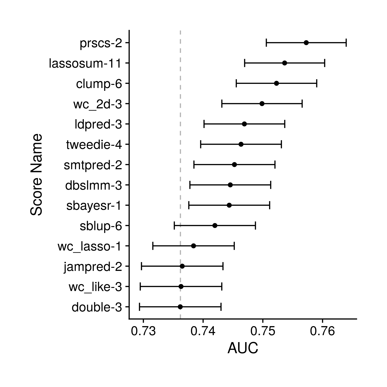
Figure 8.1: Tuning AUC Plot
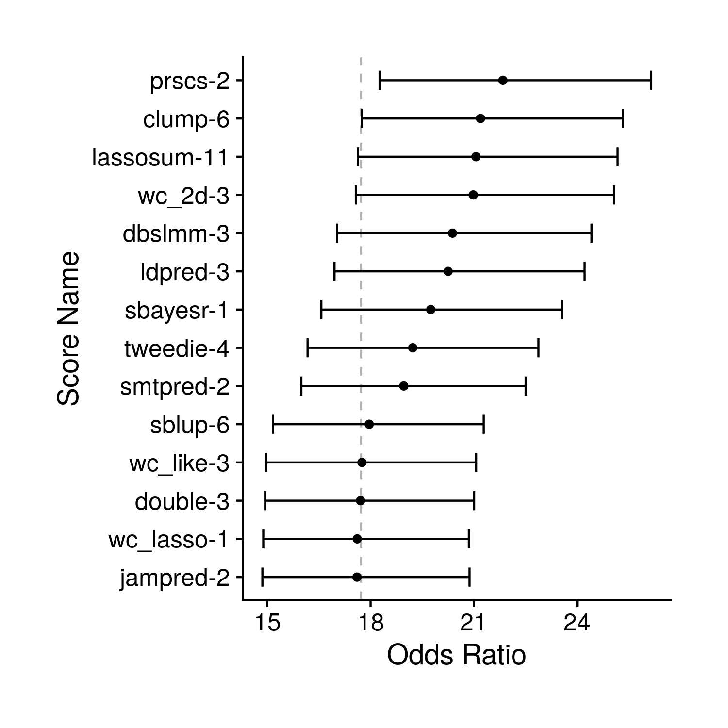
Figure 8.2: Tuning OR Plot
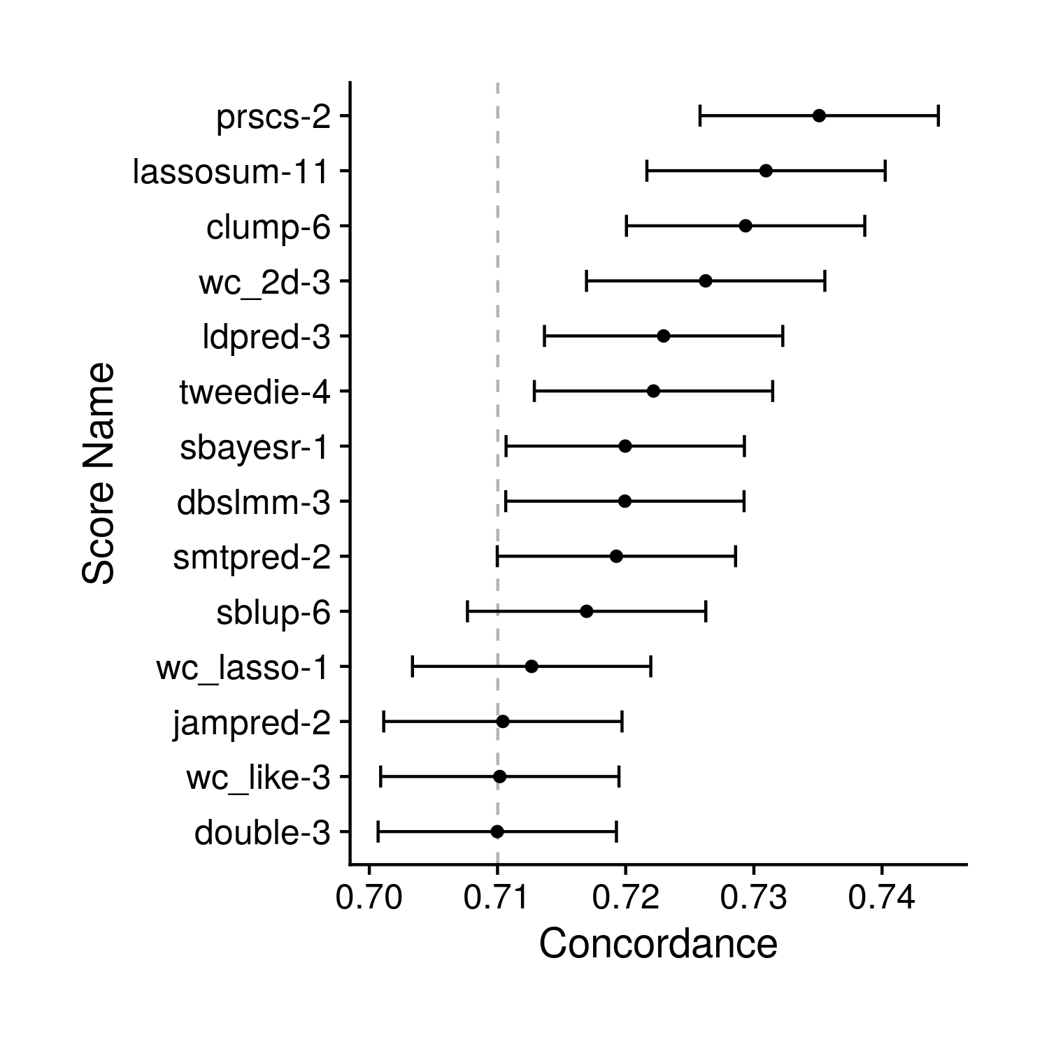
Figure 8.3: Tuning Concordance Plot
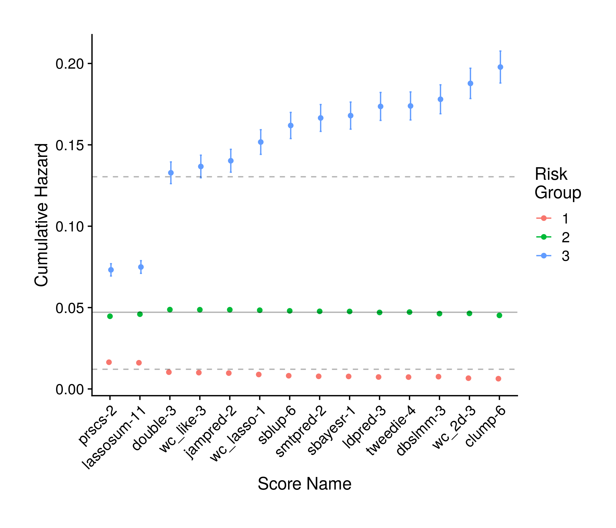
Figure 8.4: Tuning Kaplan-Meir Analysis Plot
For all plots please see: https://wcm.box.com/s/h4xrik195rdp57a0hyhjdkgf55kcju0j .