13 Lifestyle and Medications
13.1 Lifestyle Modifcations
13.1.1 Getting the Statistics
The larger project up this point has focused on either assessing the predictive accuracy of polygenic risk scores or chracterizing their component weights. In this section we add a third aim, translating polygenic risk scores to improved clinical outcomes (i.e. decrease number of disease events in a sample of individuals) via a direct clinical action. In other words the goal is to show the viability of a scenario in which you go to an appointment, doctor notcies you have a high PGS, and gives you X which thereby reduces your disease risk and effectively prevents some negative outcome.
The first class of actions investigated that may provide this PGS-linked decrease in disease risk are lifestyle modifications. Numerous papers have previously shown that individuals with high PGS experience greater drops in disease risk from a lifestyle modification than individuals with a low PGS. To replicate these results, I first pulled a handful of lifestyle measurements that the UK Biobank has to offer. While there are many different ways to proceed next, specifically defining disease risk, I followed previous examples and the most interpretable approach and classified the PRS risk as a direct grouping of PRS, not the model predications, and defined risk as the simple rate of incidence, or the number of events that occured in this study’s time frame divided by the total number of individuals. The groups of the lifestyle measure was manually completed in attempt to make the same sub-sample sizes as the PGS (1st quintile, 2-4th quintiles, 5th quintile).
An additional note to this process, that originally almost escaped me, the disease labels under analysis must be altered. Since we don’t want a disease diagnosis to occur that then changes the likelihood of lifestyle modifications, all individuals that were diagnosed before the time the lifestyles were measures, were omitted.
All lifestyle and disease combinations were assessed in this 3x3 grouping process. Those that visually appeared to contain a distinct pattern of greater disease risk reduction in the high PGS compared to low PGS groups were classified as such.
The code to compute the incidences, with the set-up identical to the primary testing script being removed for readability, is as follows:
    ###########################################################
    #                    INCIDENCE               #
    ###########################################################

    #forget everything just do prs and raw incidence
    #3,7,9

    #BASE ###############################
    get_se <- function(x){
      y <- sum(x)/length(x)
      sqrt((y*(1-y))/length(x))
    }
    get_arr_se <- function(x,y){
      a <- sum(x)
      b <- sum(y)
      n1 <- length(x)
      n2 <- length(y)
      se <- sqrt( ((a/n1)*(1-a/n1))/n1 + ((b/n2)*(1-b/n2))/n2 )
      return(se)
    }
    get_prev <- function(x){sum(x)/length(x)}
    prs_groups <- rep(1, nrow(df_test))
    prs_groups[df_test$score < quantile(df_test$score, 0.2)] <- 0
    prs_groups[df_test$score > quantile(df_test$score, 0.8)] <- 2
    #do manual:

    cont_tables <- rep(list(matrix(0, nrow = 3, ncol = 3)), ncol(mod_factors))
    se_cont_tables <- rep(list(matrix(0, nrow = 3, ncol = 3)), ncol(mod_factors))
    quants_list <- rep(list(NA), ncol(mod_factors))
    se_arr <- rep(list(c(NA, NA, NA)), ncol(mod_factors))

    for(i in 1:ncol(mod_factors)){
      use_mod <- mod_factors[!is.na(mod_factors[,i]), i]
      quants <- quantile(use_mod, c(0.2, 0.8))
      if(i == 3 | i ==7){
        quants <- c(0,2)
      } else if (i==9){
        quants <- c(1,3)
      }
      quants_list[[i]] <- quants

      use_pheno <- df_test$pheno[!is.na(mod_factors[,i])]
      use_prs <- prs_groups[!is.na(mod_factors[,i])]
      for(j in 0:2){
        cont_tables[[i]][1,j+1] <- get_prev(use_pheno[use_prs == j & use_mod <= quants[1]])
        cont_tables[[i]][2,j+1] <- get_prev(use_pheno[use_prs == j & use_mod > quants[1] & use_mod < quants[2]])
        cont_tables[[i]][3,j+1] <- get_prev(use_pheno[use_prs == j & use_mod >= quants[2]])

        se_cont_tables[[i]][1,j+1] <- get_se(use_pheno[use_prs == j & use_mod <= quants[1]])
        se_cont_tables[[i]][2,j+1] <- get_se(use_pheno[use_prs == j & use_mod > quants[1] & use_mod < quants[2]])
        se_cont_tables[[i]][3,j+1] <- get_se(use_pheno[use_prs == j & use_mod >= quants[2]])

        se_arr[[i]][j+1] <- get_arr_se(use_pheno[use_prs == j & use_mod <= quants[1]], use_pheno[use_prs == j & use_mod >= quants[2]])
      }

    }

names(cont_tables) <- colnames(mod_factors)
names(se_cont_tables) <- colnames(mod_factors)
names(quants_list) <- colnames(mod_factors)

final_obj <- list("cont_tables" = cont_tables, "se_cont_tables" = se_cont_tables, "se_arr" = se_arr)

saveRDS(final_obj, paste0("final_stats/", author, "_arr_data.RDS"))
saveRDS(quants_list, "mod_quants.RDS")
I should now note two changes that are included in this code, but were not originally thought of. First, to reduce confounding, the polygenic risk score was adjusted for age, sex, and the top ten genetic principal components (all of the base covariates). The adjustment was specifically made by taking the residuals in a basic linear regression. Second, fisher’s exact test was carried out on each iteration and within each polygenic risk score group. In each test the predicted positive are those in the high risk lifestyle group and the not predicted positive are those in the low risk lifestyle group. The p-values and odds ratios from these tests were stored for later plotting.
13.1.2 Plotting
Plots of the lifestyle modifications are fortunately very simple. The only plot form involves a grouped bar plot 3 bars in each. While I collect the data across all diseases (and even attempt to form a plot), nothing looks very good on this large (23 disease) scale, and so I do not make any overall plots. An example of the output plot is shown below.
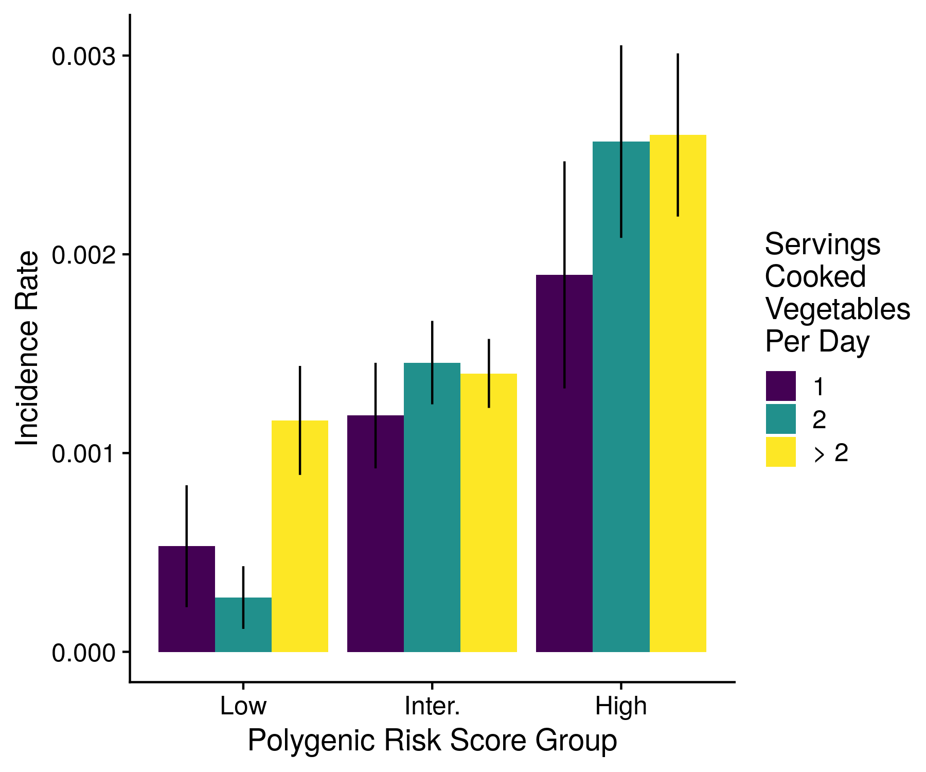
Figure 13.1: An example of the lifestyle modifications plot
And the code for making this style of plot is below. I specifically am only plotting the lifestyle and disease combinations that are deemed significant. I have not found any statistically pure way to find significancy among three p-values and have therefore taken a tri-comparison.
library(stringr)
library(ggplot2)
library(cowplot)
library(pROC)
library(reshape2)
library(rmda)
theme_set(theme_cowplot())


convert_names <- function(x, the_dict = method_dict){
  y <- rep(NA, length(x))
  for(i in 1:length(x)){
    if(x[i] %in% the_dict[,1]){
      y[i] <- the_dict[the_dict[,1] == x[i], 2]
    }
  }
  return(y)
}

method_names <- read.table("local_info/method_names", stringsAsFactors = F)
disease_names <- read.table("local_info/disease_names", stringsAsFactors = F, sep = "\t")

method_dict <- read.table("local_info/method_names", stringsAsFactors = F)
author_dict <- read.table("local_info/disease_names", stringsAsFactors = F, sep = '\t')

mod_names <- read.table("local_info/mod_splits.txt", stringsAsFactors = F, sep = "\t")

all_authors <- unique(str_split(list.files("test_results/", "class_data"), "_", simplify = T)[,1])
if(any(all_authors == "Xie")){
  all_authors <- all_authors[-which(all_authors == "Xie")]
}

#plot_authors
#plot_vars

keep_factors <- c("days_mod_activity", "smoking_status", "time_tv", "vitamin_d", "cook_veg", "alcohol_intake", "time_summer")
all_mod_df <- list()
all_supp_df <- list()
best_supp_quals <- list()
big_count <- 1
best_count <- 1

for(author in all_authors){

    res <- readRDS(paste0("test_results/", author, ".arr_data.RDS"))
    all_mod_factors <- list()
    single_supp_df <- list()

    #rows are mod risk factor
    #cols are prs risk group

    #for(i in which(names(res[[1]]) %in% keep_factors)){
    for(i in 1:length(res[[1]])){
      df <- data.frame(res[["cont_tables"]][[i]])
      sedf <- data.frame(res[["se_cont_tables"]][[i]])
      fishp <- res[["fish_stat"]][res[["fish_stat"]]$mod_factor == names(res[[1]])[i],1]
      fishor <- res[["fish_stat"]][res[["fish_stat"]]$mod_factor == names(res[[1]])[i],2]

      single_supp_df[[i]] <- as.data.frame(t(as.data.frame(signif( c(as.numeric(res[[1]][[i]]), fishp, fishor), 3))))
      colnames(single_supp_df[[i]]) <- c("prs lo - mod lo", "prs lo - mod inter", "prs lo - mod hi",
                                    "prs inter - mod lo", "prs inter - mod inter", "prs inter - mod hi",
                                    "prs hi - mod lo", "prs hi - mod inter", "prs hi - mod hi",
                                    "pval - lo", "pval - inter", "pval - hi", "or - lo", "or - inter", "or - hi")
      single_supp_df[[i]]$mod_factor <- names(res[[1]])[i]
      single_supp_df[[i]]$author <- author

      colnames(df) <- c("prs_lo", "prs_inter", "prs_hi")
      df <- melt(df)
      df$mod_group <- rep(as.character(mod_names[which(names(res[[1]])[i] == mod_names[,1]), 3:5]), 3)

      colnames(sedf) <- c("prs_lo", "prs_inter", "prs_hi")
      sedf <- melt(sedf)
      df$se <- sedf$value

      df$mod_group <- factor(df$mod_group, levels = mod_names[which(names(res[[1]])[i] == mod_names[,1]), 3:5])


      mod_drop <- df$value[seq(1,9,3)] - df$value[seq(3,9,3)]

      the_plot <- ggplot(df, aes(variable, value, fill = mod_group)) +
        geom_bar(position = position_dodge(), stat="identity") +
        geom_errorbar(aes(ymin = value - se, ymax = value + se), position = position_dodge(0.9), width = 0) +
         labs (x = "Polygenic Risk Score Group", y = "Incidence Rate",
               caption = paste("P-Vals:",  paste(as.character(signif(fishp, 3)), collapse = ", "))) +
        scale_x_discrete(labels = c("Low", "Inter.", "High")) +
        scale_fill_viridis_d(name = gsub("_", "\n", mod_names[which(names(res[[1]])[i] == mod_names[,1]),2]))

      #plot(the_plot)
      #ggsave(paste0("mod_factor_plots/", tolower(author), ".", poss_eps[kk], ".", mod_names[i,1], ".png"),
      #       the_plot, "png", height=5, width=6)
      if(all(fishp < 0.05) | sum(fishp < 0.005) == 2 | any(fishp[c(1,3)] < 0.0005)){
        if(abs(mod_drop[3]) > abs(mod_drop[1])){
          if(all(df$value > 0)){
          ggsave(paste0("great_mod_factor_plots/", tolower(author), ".", names(res[[1]])[i], ".png"),
                 the_plot, "png", height=4.5, width=5)
          best_supp_quals[[best_count]] <- c(author, names(res[[1]])[i])
          best_count <- best_count + 1
          }
        }
      }

      all_mod_factors[[i]] <- df
      all_mod_factors[[i]]$mod_factor <- names(res[["cont_tables"]])[i]
      all_mod_factors[[i]]$author <- author

    }


    all_mod_df[[big_count]] <- all_mod_factors
    all_supp_df[[big_count]] <- single_supp_df
    big_count <- big_count + 1

}


redo_list <- list()
k <- 1
for(i in 1:length(all_supp_df)){
  for(j in 1:length(all_supp_df[[i]])){
    if(!is.null(all_supp_df[[i]][[j]])){
      redo_list[[k]] <- all_supp_df[[i]][[j]]
      k <- k + 1
    }
  }
}

big_df <- do.call("rbind", redo_list)

keep_rows <- do.call("rbind", best_supp_quals)
best_df <- big_df[paste0(big_df$author, "_", big_df$mod_factor) %in% paste0(keep_rows[,1], "_", keep_rows[,2]),]
best_df$disease <- convert_names(best_df$author, author_dict)
best_df$mod_name <- convert_names(best_df$mod_factor, mod_names)

for(i in 1:9){
  best_df[,i] <- signif(best_df[,i], 2)
}

best_df <- best_df[best_df$mod_factor != "cook_veg",]
best_df$mod_name <- gsub("_", " ", best_df$mod_name)
supp1 <- best_df[,c(18, 19, 1:9)]
supp2 <- best_df[,c(18, 19,  10:15)]

supp1$mod_name[supp1$mod_name == "Pieces Fruit Eaten Per Day"] <- "Fruit"
supp1$mod_name[supp1$mod_name == "Hours per Day Watch TV"] <- "TV"
supp1$mod_name[supp1$mod_name == "Processed Meat Intake"] <- "Meat"
supp1$mod_name[supp1$mod_name == "Glasses of Water Per Day"] <- "Water Intake"
supp1$mod_name[supp1$mod_name == "Days Mod. Activity Per Week"] <- "Mod. Activity"
supp1$mod_name[supp1$mod_name == "Hours per Day Driving"] <- "Driving"
supp1$mod_name[supp1$mod_name == "Tbsp Raw Veg. Per Day"] <- "Vegetable"
supp1$mod_name[supp1$mod_name == "Alcohol Consumed"] <- "Alcohol"
supp1$mod_name[supp1$mod_name == "Min. Walked Per Day"] <- "Min. Walked"

supp2$mod_name[supp2$mod_name == "Pieces Fruit Eaten Per Day"] <- "Fruit"
supp2$mod_name[supp2$mod_name == "Hours per Day Watch TV"] <- "TV"
supp2$mod_name[supp2$mod_name == "Processed Meat Intake"] <- "Meat"
supp2$mod_name[supp2$mod_name == "Glasses of Water Per Day"] <- "Water Intake"
supp2$mod_name[supp2$mod_name == "Days Mod. Activity Per Week"] <- "Mod. Activity"
supp2$mod_name[supp2$mod_name == "Hours per Day Driving"] <- "Driving"
supp2$mod_name[supp2$mod_name == "Tbsp Raw Veg. Per Day"] <- "Vegetable"
supp2$mod_name[supp2$mod_name == "Alcohol Consumed"] <- "Alcohol"
supp2$mod_name[supp2$mod_name == "Min. Walked Per Day"] <- "Min. Walked"


write.table(supp1, paste0("supp_tables/mod_factor.vals.txt"), col.names = T, row.names = F, quote = F, sep = "\t")
write.table(supp2, paste0("supp_tables/mod_factor.sigs.txt"), col.names = T, row.names = F, quote = F, sep = "\t")


# for(uval in unique(big_df$mod_factor)){
#   small_df <- big_df[big_df$mod_factor == uval,]
#   small_df <- small_df[,-which(colnames(small_df) == "mod_factor")]
#   small_df$author <- convert_names(small_df$author, author_dict)
#   small_df <- small_df[,c(10,1:9)]
#   new_df <- as.data.frame(rbind(str_split(colnames(small_df), "-", simplify = T)[,1],
#                                 str_split(colnames(small_df), "-", simplify = T)[,2]), stringsAsFactors = F)
#   colnames(new_df) <- colnames(small_df)
#   small_df <- rbind(new_df, small_df)
#   write.table(small_df, paste0("supp_tables/mod_factor.", uval, ".txt"), col.names = F, row.names = F, quote = F, sep = "\t")
# }
13.2 Medications
13.2.1 Set Up
In truth, this entire section started out with the hopes of it being a much larger independent project. This fact can hopefully explain why the data is organized in a much more sophistacted manner than necessary. The underlying motivation has remained the same throughout however, determine whether the efficacy of a medication is affected by the polygenic risk score a person has. This is essentially the same premise of the lifestyle analysis, although with prescription data at various timepoints and various dosages the analysis gets a bit more complex.
To start this analysis we need to define the sub-cohorts of people we want to analyze. While we could simply analyze whether a medication changes how likely you are to get a disease, more often than not that is not how a medication is designed. Rather, a medication is designed to reduce the negative outcomes of a disease once it is known and diagnosed. Therefore, several endpoints that do not just include disease onset were included. Under these analyses the sub-cohort contained only people that were diagnosed with a relavent illness, thereby setting up an artifical study that someone could create if they were going to go through the steps of getting an IRB, enrolling the relavent participants, following their outcomes and doing the analysis. The script used to get these endpoints is exactly the same as the one used to define the primary disease phenotypes, so I will not repeat it here. The endpoints under consideration and their definitions are as follows:
x <- read.table("/home/quenton/Academics/doc_score/med_scripts/all_endpoints", stringsAsFactors=F, sep="\t", fill =T)
print(x)
## V1 V2 V3 V4
## 1 author endpt1 endpt2 endpt3
## 2 Bentham dependence fatigue
## 3 Christophersen disese_onset stroke death_cardio
## 4 Demenais disese_onset
## 5 Dubois disese_onset
## 6 Gormley disese_onset
## 7 IMSGC disese_onset dependence fatigue
## 8 Kottgen disese_onset
## 9 Liu-1 disese_onset disease_of_intestine
## 10 Liu-2 disese_onset disease_of_intestine
## 11 Mahajan disese_onset diabetes_complication_2 death_diabetes
## 12 Malik disese_onset death_early
## 13 Michailidou disese_onset death_bc death_early
## 14 Namjou liver_failure death_liver death_early
## 15 Nikpay disese_onset myocardial_infarction heart_failure
## 16 Okada disese_onset
## 17 Onengut disese_onset diabetes_complication_1 death_diabetes
## 18 Phelan disese_onset death_oc death_early
## 19 Schumacher disese_onset death_pc death_early
## 20 Shah disese_onset death_cardio death_early
## 21 Wray disese_onset
## V5 V6 V7
## 1 endpt4 endpt5 endpt6
## 2
## 3 death_early
## 4
## 5
## 6
## 7 death_ms death_early
## 8
## 9
## 10
## 11 death_early
## 12
## 13
## 14
## 15 arrhythmia death_cardio death_early
## 16
## 17 death_early
## 18
## 19
## 20
## 21x <- read.table("/home/quenton/Academics/doc_score/med_scripts/endpoint_def", stringsAsFactors=F, sep="\t", fill =T)
print(x)## V1 V2 V3 V4 V5 V6
## 1 author name sex cancer noncancer icd9
## 2 dependence dependence A <NA> <NA> V46
## 3 fatigue fatigue A <NA> <NA> 7807
## 4 disease_of_intestine disease_of_intestine A <NA> <NA> 560
## 5 diabetes_complication_1 diabetes_complication_1 A <NA> <NA> <NA>
## 6 diabetes_complication_2 diabetes_complication_2 A <NA> <NA> <NA>
## 7 liver_failure liver_failure A <NA> <NA> 5739
## 8 myocardial_infarction myocardial_infarction A <NA> <NA> 410
## 9 arrhythmia arrhythmia A <NA> <NA> 426|427
## V7 V8 V9
## 1 icd10 opcs meds
## 2 R263|Z99 <NA> <NA>
## 3 R53 <NA> <NA>
## 4 K63 <NA> <NA>
## 5 E100|E101|E102|E103|E104|E105|E106|E107|E108 <NA> <NA>
## 6 E110|E111|E112|E113|E114|E115|E116|E117|E118|E119 <NA> <NA>
## 7 K72 <NA> <NA>
## 8 I21 <NA> <NA>
## 9 I44|I45|I47|I48|I49 <NA> <NA>Once the identities of the individuals in each sub-cohort are realized, we must find all of the medications that could effect the respective outcome. This step requires understanding how UK Biobank organized the medication data. A full description of the data is here: https://biobank.ndph.ox.ac.uk/showcase/showcase/docs/primary_care_data.pdf. In short, the prescriptions in general practices that are electronically linked to the UK Biobanked are compiled together. If a UK Biobank participant changed general practices and went to a non-linked practice then there would be an artifical gap in the data. The specific form of the prescription collected include the date, BNF code and the raw text of the prescription. In order to increase the number of medications that apply to a group and limit the problems of identifying the text of a medication name, the medications are grouped by BNF code. Moving ahead in the medication analysis, for each sub-cohort all possible medications (BNF codes) are gathered and simply counted. If there are more than 50 people who take a medication and reach the sub-cohort endpoint then the name of the medication is kept for later analysis.
The exact code that carries out this sample sizing is below. The crux of it is that a sub-cohort is briefly assembled, those EIDs are used to subset all script data via fgrep on the command line, then the subset script is read beack into R and counted. There is a slightly different script for disease_onset and non-disease_onset.
library(data.table)

#This script is for generating the med info for the general onset of disease endpoint

#author <- "christophersen"
author <- tolower(commandArgs(trailingOnly=TRUE))

dates <- read.table(paste0("~/athena/doc_score/analyze_score/construct_defs/pheno_defs/time.", author, ".txt.gz"), stringsAsFactors=F)
for(i in 1:ncol(dates)){
  if(i %in% c(1,2,6)){
    dates[dates[,i] == "__________", i] <- "2020-12-31"
    dates[,i] <- as.Date(dates[,i], "%Y-%m-%d")
  } else {
    dates[dates[,i] == "__________", i] <- "31/12/2020"
    dates[,i] <- as.Date(dates[,i], "%d/%m/%Y")
  }
}
pheno_time <- dates[,-ncol(dates)]

eid <- read.table("~/athena/doc_score/analyze_score/construct_defs/eid.csv", stringsAsFactors=F, header=T, nrows = nrow(pheno_time))


#####################################################
#PHENO GROUPS #######################################

  check_inds <- which(apply(pheno_time, 1, function(x) any(x != "2020-12-31")))

  sub_pheno <- apply(pheno_time[check_inds,], 1, min)
  sub_eid <- eid[check_inds,]
  #get the eids and dates of people with disease

  write.table(sub_eid, "meds_in_interval/good_eids", row.names = F, col.names = F, quote = F)
  system("zcat ~/athena/ukbiobank/gp/gp_scripts.txt.gz | fgrep -w -f meds_in_interval/good_eids > meds_in_interval/sub_gp")
  if(file.info("meds_in_interval/sub_gp")$size > 0){

    #sub_gp <- read.table("sub_gp", stringsAsFactors=F, sep = '\t', fill = T)
    sub_gp <- as.data.frame(fread("meds_in_interval/sub_gp"))
    sub_gp[,3] <- as.Date(sub_gp[,3], "%d/%m/%Y")
    sub_gp <- sub_gp[sub_gp[,3] > as.Date("1999-01-01"),]

    #add in the medications that occur before a given date
    #sub_eid are individuals who go on to get the disease
    all_good_meds <- list()
    for(k in 1:length(sub_eid)){
      if(sub_eid[k] %in% sub_gp[,1]){ #condition that meds are taken by eid and those meds were prescribed before date of diagnosis
        all_good_meds[[k]] <- unique(substr(sub_gp[sub_gp[,1] == sub_eid[k] & sub_gp[,3] < sub_pheno[k],5], 1, 8))
      } else {
        all_good_meds[[k]] <- "none"
      }
    }

    #do the table to get amount of people on a medication
    final_meds <- sort(table(unlist(all_good_meds)), decreasing=T)
    final_meds <- final_meds[final_meds > 50 & names(final_meds) != "none" & final_meds != ""]

    saveRDS(final_meds, paste0("meds_in_interval/", author, ".disease_onset.RDS"))
  }

system("rm meds_in_interval/sub_gp")

#NOTE: All of the numbers are the number of people with med and either cases or cases then death
Once the sub-cohort, endpoint and possible medications under analysis are all set it is time to actually do the analysis. The first step is set-up, which compiled the very simple survival data frame. There is a row for each individual with a start and end date, with a phenotype marker of endpoint or censor. The code is very similar to what has been used in previous testing sections but I will still include the code here:
library(survival)
library(pROC)
library(epitools)


args <- commandArgs(trailingOnly=TRUE)
author <- args[1]
endpoint <- args[2]
#author <- "Christophersen"
#endpoint <- "disease_onset"


#get scores
all_scores <-  readRDS(paste0("~/athena/doc_score/do_score/final_scores/all_score.", tolower(author), ".RDS"))
all_eid <- read.table("~/athena/doc_score/do_score/all_specs/for_eid.fam", stringsAsFactors=F)
train_eid <- read.table(paste0("~/athena/doc_score/qc/cv_files/train_eid.0.8.txt"), stringsAsFactors=F)
test_eid <- read.table(paste0("~/athena/doc_score/qc/cv_files/test_eid.0.2.txt"), stringsAsFactors=F)
new_eid <- rbind(train_eid, test_eid)
all_scores <- all_scores[all_eid[,1] %in% new_eid[,1],]
eid <- all_eid[all_eid[,1] %in% new_eid[,1],1]


#Normalize the scores
scores <- all_scores[,grepl(tolower(author), colnames(all_scores))]
scores <- scores[,apply(scores, 2, function(x) length(unique(x)) > 3)]
scores <- apply(scores, 2, function(x) (x-mean(x)) / (max(abs((x-mean(x)))) * 0.01) )


get_pheno <- function(author, keep_score){
  #Read in the phenotypes, order is: cancer sr, noncancer sr, icd9, icd10, oper, meds
  #selfasses date: 2018-11-22; hesin date: 21/01/2000
  if( any(grepl(tolower(author), list.files("../endpoints/disease_endpoints/"))) ){
    dates <- read.table(paste0("/home/kulmsc/athena/med_surv_study/endpoints/disease_endpoints/time.", tolower(author), ".txt.gz"), stringsAsFactors=F)
  } else if(grepl("death", author)){
    dates <- read.table(paste0("/home/kulmsc/athena/med_surv_study/endpoints/death_endpoints/time.", tolower(author), ".txt.gz"), stringsAsFactors=F)
  } else {
    if(author == "heart_failure"){
      dates <- read.table(paste0("/home/kulmsc/athena/med_surv_study/endpoints/disease_endpoints/time.shah.txt.gz"), stringsAsFactors=F)
    } else if(author == "stroke"){
      dates <- read.table(paste0("/home/kulmsc/athena/med_surv_study/endpoints/disease_endpoints/time.malik.txt.gz"), stringsAsFactors=F)
    } else {
      dates <- read.table(paste0("/home/kulmsc/athena/med_surv_study/endpoints/other_endpoints/time.", tolower(author), ".txt.gz"), stringsAsFactors=F)
    }
  }

  for(i in 1:ncol(dates)){
    if(any(grepl("-", dates[,i]))){
      dates[dates[,i] == "__________", i] <- "2020-12-31"
      dates[,i] <- as.Date(dates[,i], "%Y-%m-%d")
    } else {
      dates[dates[,i] == "__________", i] <- "31/12/2020"
      dates[,i] <- as.Date(dates[,i], "%d/%m/%Y")
    }
  }

  dates <- dates[,1:4]

  dates <- apply(dates, 1, min)
  dates[dates == as.Date("2020-12-31")] <- NA

  pheno <- rep(0, length(dates))
  pheno[!is.na(dates)] <- 1

  #Read in the eids used that are the same order as the pheno and dates, then subset the pheno and dates accordingly
  pheno_eids <- read.table("~/athena/doc_score/analyze_score/construct_defs/eid.csv", header = T)
  pheno_eids <- pheno_eids[order(pheno_eids[,1]),]
  pheno_eids <- pheno_eids[-length(pheno_eids)]
  if(keep_score){
    scores <- scores[eid %in% pheno_eids,]
  } else {
    scores <- NULL
  }
  eid <- eid[eid %in% pheno_eids]
  dates <- dates[pheno_eids %in% eid]
  pheno <- pheno[pheno_eids %in% eid]
  pheno_eids <- pheno_eids[pheno_eids %in% eid]
  dates <- dates[order(pheno_eids)[rank(eid)]]
  pheno <- pheno[order(pheno_eids)[rank(eid)]]

  return(list(dates, pheno, pheno_eids, scores))
}

base_info <- get_pheno(author, TRUE)
if(endpoint != "disease_onset"){
  end_info <- get_pheno(endpoint, FALSE)
}


dates <- base_info[[1]]
pheno <- base_info[[2]]
eid <- base_info[[3]]
scores <- base_info[[4]]


#Read in the base covars
covars <- readRDS("~/athena/doc_score/analyze_score/get_covars/base_covars.RDS")
covars <- covars[covars[,1] %in% eid,]
covars <- covars[order(covars[,1])[rank(eid)],]


#Set up survival analysis data frame
#Artifically decide start date is 1999, that way all are even, if date is prior then remove it
#The current maximum date possible is 31 May 2020
death <- read.table("~/athena/ukbiobank/hesin/death.txt", stringsAsFactors=F, header = T)
death[,5] <- unlist(lapply(death[,5], function(x) paste0(strsplit(x, "/")[[1]][3], "-", strsplit(x, "/")[[1]][2], "-", strsplit(x, "/")[[1]][1])))
death <- death[!duplicated(death[,1]),]
death <- death[death[,1] %in% eid,]
add_on <- death[1,]
add_on[5] <- ""
add_eid <- eid[!(eid %in% death[,1])]
add_on <- add_on[rep(1, length(add_eid)),]
add_on$eid <- add_eid
death <- rbind(death, add_on)
death <- death[order(death[,1])[rank(eid)],]

censor <- read.table("~/athena/doc_score/analyze_score/get_covars/covar_data/censor_covars", stringsAsFactors=F, header = T, sep = ",")
censor <- censor[censor[,1] %in% eid,]
censor <- censor[order(censor[,1])[rank(eid)],]


#set up start and end dates
start_date <- rep("1999-01-01", length(eid))
end_date <- rep("2020-05-31", length(eid))
end_date[censor[,2] != ""] <- censor[censor[,2] != "", 2]
end_date[death[,5] != ""] <- death[death[,5] != "", 5]
end_date[!is.na(dates)] <- dates[!is.na(dates)]


is_death_date <- rep(0, nrow(scores))
is_death_date[death[,5] != "" & pheno == 0] <- 1
surv_df <- data.frame(time = as.numeric(as.Date(end_date) - as.Date(start_date)), start_date, end_date, pheno, is_death_date, covars)

if(endpoint != "disease_onset"){

  surv_df <- surv_df[surv_df$pheno == 1,]
  surv_df$start_date <- surv_df$end_date
  surv_df$end_date <- rep("2020-05-31", nrow(surv_df))

  real_end_date <- end_info[[1]][end_info[[3]] %in% surv_df$eid]
  real_eid <- end_info[[3]][end_info[[3]] %in% surv_df$eid]

  surv_df$end_date[!is.na(real_end_date)] <- real_end_date[!is.na(real_end_date)]
  surv_df$pheno <- 0
  surv_df$pheno[!is.na(real_end_date)] <- 1

  surv_df$time <- as.numeric(as.Date(surv_df$end_date) - as.Date(surv_df$start_date))
}

real_eid <- eid[surv_df$time > 0]
scores <- scores[surv_df$time > 0,]
surv_df <- surv_df[surv_df$time > 0,]


author_defs <- read.table("~/athena/doc_score/analyze_score/descript_defs/author_defs", stringsAsFactors=F, header=T)
subset_sex <- author_defs$sex[author_defs$author == author]
if(subset_sex == "F"){
  real_eid <- real_eid[surv_df$sex == 0]
  scores <- scores[surv_df$sex == 0,]
  surv_df <- surv_df[surv_df$sex == 0,]
} else if(subset_sex == "M"){
  real_eid <- real_eid[surv_df$sex == 1]
  scores <- scores[surv_df$sex == 1,]
  surv_df <- surv_df[surv_df$sex == 1,]
}

saveRDS(list(surv_df, scores, real_eid), paste0("surv_dfs/", author, ".", endpoint, ".RDS"))
13.2.2 Meications
Next, we need to add the medications into the survival dataframe. Going back to project origins, I include far more detailed information than necessary, specifically, the level of dosage for each segment of time. For example, each prescription is translated to a dosage and pill value. So “Dosulepin 25mg capsules 168 caps” would be coverted to 25mg level of dosage and 168 pills. A somewhat involved “natural language processing” set of rules will try to match a number next to the mg/ml/g unit to dosage and pills/caps/etc. to the pills. A very rough estimate of 1 pill per day is used, and the dosage is held constant for each day (although in some cases the dosage is divided across all days if the text states). This data is then organized to a row in the survival dataframe, with the starting date of the prescription used as reference. After going across all prescriptions for an individual, a final check is made to make sure prescriptions do not overlap and extend beyond the end of the larger dataframe.
The entire code that pulls out the dosage and pills, then correctly determines how to organize the survival dataframe with this prescription data follows:
library(stringr)
library(data.table)
options(warn=2)

#MUST EDIT THIS!!!!!!!!!!!

#author <- "Christophersen"
#endpoint <- "death_early"
args <- commandArgs(trailingOnly=TRUE)
author <- args[1]
endpoint <- args[2]

get_first <- function(drug_string){
  #val <- strsplit(drug_string, " ")[[1]][1]
  if(grepl("[0-9]", substr(drug_string, 1, 1))){
    val <- unlist(regmatches(drug_string, gregexpr('\\(?[0-9,.]+', drug_string)))[1]
    val <- gsub("(", "", val, fixed=T)
  } else {
    val <- NA
  }
  return(val)
}

get_val <- function(drug_string, split_by){
  if(grepl(split_by, drug_string)){
    drug_string <- trimws(str_split(drug_string[1], split_by)[[1]][1])
    if(grepl("[0-9]", substr(drug_string, nchar(drug_string), nchar(drug_string)))){
      drug_num <- tail(unlist(regmatches(drug_string, gregexpr('\\(?[0-9,.]+', drug_string))), 1) #works for everything but commas
      if(grepl(",", drug_num)){
        drug_num <- tail(strsplit(drug_num, ",")[[1]], 1)
      }
      drug_num <- gsub("(", "", drug_num, fixed=T)
    } else {
      drug_num <- NA
    }
  } else {
    drug_num <- NA
  }
  return(drug_num)
}


surv_objs <- readRDS(paste0("surv_dfs/", author, ".", endpoint, ".RDS"))
script_eids <- read.table("script_eids", stringsAsFactors=F)

surv_scores <- surv_objs[[2]][surv_objs[[1]]$eid %in% script_eids[,1],] #I do not include scores in this process, in part to keep things smaller
surv_df <- surv_objs[[1]][surv_objs[[1]]$eid %in% script_eids[,1],]
surv_df$start_time <- 0
surv_df$med_amt <- 0
surv_df$start_date <- as.Date(surv_df$start_date)
surv_df$end_date <- as.Date(surv_df$end_date)
surv_df$dosage <- 0

surv_df <- surv_df[surv_df$start_date < surv_df$end_date,]


if(file.exists(paste0("../endpoints/meds_in_interval/", tolower(author), ".", tolower(endpoint), ".RDS"))){
  med_vec <- readRDS(paste0("../endpoints/meds_in_interval/", tolower(author), ".", tolower(endpoint), ".RDS"))
} else {
  med_vec <- readRDS(paste0("../endpoints/meds_in_interval/", tolower(author), ".", tolower(endpoint), ".spec.RDS"))
}


if(length(med_vec) > 0){

  #Iterating over each medication
  #for(i in 1:min(10, length(med_vec))){
  for(i in 1:length(med_vec)){
    #final_name <- paste0("med_files/", author, "/", author, ".", names(med_vec[i]), ".", endpoint, ".df.RDS")
    final_name <- paste0("med_dfs/", author, ".", endpoint, ".",  names(med_vec[i]), ".RDS")
    if(file.exists(final_name)){
      print(i)
    } else {
    print(paste("med_vec", i))
    write.table(names(med_vec)[i], "temp_med_name", row.names = F, col.names = F, quote = F)
    system("zcat ~/athena/ukbiobank/gp/gp_scripts.txt.gz | fgrep -w -f temp_med_name | grep -ax '.*'> sub_gp_script2")

    #sub_gp <- read.table("sub_gp_script", stringsAsFactors=F, sep = '\t')
    sub_gp <- as.data.frame(fread("sub_gp_script2", quote = "^")) #66630
    sub_gp <- sub_gp[grep(paste0("^", names(med_vec)[i]), sub_gp[,5]), ]
    sub_gp[,3] <- as.Date(sub_gp[,3], "%d/%m/%Y")
    #sub_gp <- sub_gp[sub_gp[,3] > as.Date("1999-01-01"),]
    sub_gp <- sub_gp[sub_gp[,1] %in% surv_df$eid,]

    ################################################################################
    #need to extract mg information ######
    ################################################################################
    print("extracting info")
    unq_med_names <- unique(sub_gp[,7])
    unq_dose_names <- unique(sub_gp[,8])

    dose_info_1 <- as.numeric(unlist(lapply(tolower(unq_med_names), get_val, "mg")))
    dose_info_2 <- as.numeric(unlist(lapply(tolower(unq_med_names), get_val, "g"))) * 1000
    dose_info_3 <- as.numeric(unlist(lapply(tolower(unq_med_names), get_val, "milli")))
    dose_info_4 <- as.numeric(unlist(lapply(tolower(unq_med_names), get_val, "ml")))

    dose_info_5 <- as.numeric(unlist(lapply(tolower(unq_dose_names), get_val, "mg")))
    dose_info_6 <- as.numeric(unlist(lapply(tolower(unq_dose_names), get_val, "g"))) * 1000
    dose_info_7 <- as.numeric(unlist(lapply(tolower(unq_dose_names), get_val, "milli")))
    dose_info_8 <- as.numeric(unlist(lapply(tolower(unq_dose_names), get_val, "ml")))

    freq_info_1 <- as.numeric(unlist(lapply(tolower(unq_dose_names), get_val, "tab")))
    freq_info_2 <- as.numeric(unlist(lapply(tolower(unq_dose_names), get_val, "cap")))
    freq_info_3 <- as.numeric(unlist(lapply(tolower(unq_dose_names), get_val, "day")))
    freq_info_4 <- as.numeric(unlist(lapply(tolower(unq_dose_names), get_val, "pack")))

    freq_info_5 <- as.numeric(unlist(lapply(tolower(unq_dose_names), get_first)))
    freq_info_5[freq_info_5 == dose_info_5] <- NA
    freq_info_5[freq_info_5 == dose_info_6] <- NA
    freq_info_5[freq_info_5 == dose_info_7] <- NA
    freq_info_5[freq_info_5 == dose_info_8] <- NA

    dose_amt <- rep(NA, nrow(sub_gp))
    pill_amt <- rep(NA, nrow(sub_gp))
    freq_amt <- rep(NA, nrow(sub_gp))

    for(j in 1:length(unq_med_names)){
      dose_amt[sub_gp[,7] == unq_med_names[j]] <- dose_info_1[j]
      dose_amt[sub_gp[,7] == unq_med_names[j] & is.na(dose_amt)] <- dose_info_2[j]
      dose_amt[sub_gp[,7] == unq_med_names[j] & is.na(dose_amt)] <- dose_info_3[j]
      dose_amt[sub_gp[,7] == unq_med_names[j] & is.na(dose_amt)] <- dose_info_4[j]
    }

    for(j in 1:length(unq_dose_names)){
      dose_amt[sub_gp[,8] == unq_dose_names[j] & is.na(dose_amt)] <- dose_info_5[j]
      dose_amt[sub_gp[,8] == unq_dose_names[j] & is.na(dose_amt)] <- dose_info_6[j]
      dose_amt[sub_gp[,8] == unq_dose_names[j] & is.na(dose_amt)] <- dose_info_7[j]
      dose_amt[sub_gp[,8] == unq_dose_names[j] & is.na(dose_amt)] <- dose_info_8[j]

      pill_amt[sub_gp[,8] == unq_dose_names[j]] <- freq_info_1[j]
      pill_amt[sub_gp[,8] == unq_dose_names[j] & is.na(pill_amt)] <- freq_info_2[j]
      pill_amt[sub_gp[,8] == unq_dose_names[j] & is.na(pill_amt)] <- freq_info_3[j]

      freq_amt[sub_gp[,8] == unq_dose_names[j]] <- freq_info_4[j]
      pill_amt[sub_gp[,8] == unq_dose_names[j] & is.na(pill_amt) & is.na(freq_amt)] <- freq_info_5[j]
      #freq_amt[(sub_gp[,8] == unq_dose_names[j]) & is.na(freq_amt) & !is.na(pill_amt) & (freq_info_5[j] != pill_amt[sub_gp[,8] == unq_dose_names[j])] <- freq_info_5[j]
    }

    freq_amt[is.na(freq_amt)] <- 1
    pill_amt <- pill_amt * freq_amt
    pill_amt[!is.na(pill_amt)][pill_amt[!is.na(pill_amt)] > quantile(pill_amt[!is.na(pill_amt)], 0.99)] <- median(pill_amt[!is.na(pill_amt)])
    pill_amt[is.na(pill_amt)] <- median(pill_amt)

    dose_amt[is.na(dose_amt)] <- mean(dose_amt, na.rm = T)
    pill_amt[is.na(pill_amt)] <- mean(pill_amt, na.rm = T)

    sub_gp$dose <- dose_amt
    sub_gp$pill <- pill_amt
    sub_gp$pill[sub_gp$pill == 0] <- 1

    ###########################################################################
    # need to create new survival df
    ###########################################################################
    print("creating new df")
    new_gp_dfs <- list()
    k <- 1
    good_to_use_eid <- unique(sub_gp[,1])[unique(sub_gp[,1]) %in% surv_df$eid]
    for(eid in good_to_use_eid){
      eid_gp <- sub_gp[sub_gp[,1] == eid,]
      eid_surv <- surv_df[surv_df$eid == eid,]
      eid_gp <- eid_gp[eid_gp[,3] < eid_surv$end_date & eid_gp[,3] > eid_surv$start_date & !is.na(eid_gp[,3]),]
      eid_surv_pheno <- eid_surv$pheno

      if(nrow(eid_gp) > 0){
        #when two prescriptions are made on one day
        if(any(duplicated(eid_gp[,3]))){
          bad_date <- eid_gp[duplicated(eid_gp[,3]),3]
          add_dose <- eid_gp$dose[duplicated(eid_gp[,3])]
          eid_gp <- eid_gp[!duplicated(eid_gp[,3]),]
          for(m in 1:length(bad_date)){
            eid_gp$dose[eid_gp[,3] == bad_date[m]] <- eid_gp$dose[eid_gp[,3] == bad_date[m]] + add_dose[m]
          }
        }

        #if presscription is made past the time of death (or phenotype?)
        past_death <- (eid_gp[,3] + eid_gp$pill) >= eid_surv$end_date
        if(any(past_death)){
          eid_gp$pill[past_death] <- as.numeric(eid_surv$end_date - eid_gp[past_death,3] - 1)
          past_death <- (eid_gp[,3] + eid_gp$pill) >= eid_surv$end_date
          if(any(past_death)){
            eid_gp <- eid_gp[!past_death,]
          }
          eid_gp <- eid_gp[eid_gp$pill > 0,]
        }

        if(nrow(eid_gp) > 0){

          eid_surv <- eid_surv[rep(1, 2+nrow(eid_gp)),]
          eid_surv$pheno <- 0

          eid_surv$start_date <- c(eid_surv$start_date[1], eid_gp[,3], eid_gp[nrow(eid_gp),3]+eid_gp$pill[nrow(eid_gp)])
          eid_surv$end_date <- c(eid_gp[1,3], eid_gp[,3]+eid_gp$pill, eid_surv$end_date[1])
          eid_surv$dosage <- c(0, eid_gp$dose, 0)
          eid_surv$time <- as.numeric(eid_surv$end_date - eid_surv$start_date)
          eid_surv$end_time <- cumsum(eid_surv$time)
          eid_surv$start_time <- c(0, cumsum(eid_surv$time)[-nrow(eid_surv)])
          eid_surv$pheno[nrow(eid_surv)] <- eid_surv_pheno

          if(any(eid_surv$end_date <= eid_surv$start_date)){
            exit()
          }

        } else {
          eid_surv$end_time <- eid_surv$time
          eid_surv$start_time <- 0
        }
      } else {
        eid_surv$end_time <- eid_surv$time
        eid_surv$start_time <- 0
      }
      new_gp_dfs[[k]] <- eid_surv
      k <- k + 1
    }

    print("finishing")
    new_gp_dfs <- do.call("rbind", new_gp_dfs)
    rest_surv_df <- surv_df[!(surv_df$eid %in% good_to_use_eid),]
    rest_surv_df$end_time <- rest_surv_df$time
    final_df <- rbind(new_gp_dfs, rest_surv_df)
    if(!all(final_df$eid %in% surv_objs[[1]]$eid)){
      print("BAD: EID SHOULD NOT BE THERE")
    }
    saveRDS(final_df, paste0("med_dfs/", author, ".", endpoint, ".",  names(med_vec[i]), ".RDS"))

    }
  }
}
13.2.3 Analysis
The last part is the actual logistic regression for each sub-cohort, endpoint and medication. You may think that with the whole, complicated survival data frame situation I would be going with a time-dependent cox proportional hazards model. I thought that too, but then I tried it and the models either do not converge at all or converge in a way that gives you crazy answers. Therefore, I just went with the tried and true logistic regression, which required me to collapse all of the time information together. Although, since this change would make the dosage feature a simple sum of all the dosages I decided to do something a little bit more advanced. I wrote a few functions that look across the time-aware dosage data and return a different dosage measurement. For example:
get_frac_time <- function(x){
   sum(x$time[x$dosage != 0])/x$end_time[nrow(x)]
}
get_mean_dose <- function(x){
   mean((x$dosage * (x$end_time - x$start_time))/x$end_time[nrow(x)])
}
get_last_3year <- function(x){
   sum(x$dosage[x$start_time > x$start_time[nrow(x)] - 365*3])
}
With the simplified data frame and the dosage measurements of note completed the only thing left to do was regress. Three regressions in total were done over three polygenic risk score groups, the first quintile, third to fourth quintile, and fifth quintile. The resulting effects from each of these 3 regressions are extracted, and saved for later. The full script that runs this dosage splitting and regression process is:
library(survival)
library(plyr)

#New idea, when doing the repeat event survival analysis make the analysis equal cases and controls
options(warn=2)

#author <- "Christophersen"
#endpoint <- "death_early"
args <- commandArgs(trailingOnly=TRUE)
author <- args[1]
endpoint <- args[2]

surv_objs <- readRDS(paste0("surv_dfs/", author, ".", endpoint, ".RDS"))

pgs_fitting <- function(df, dose_name){
  pgs_group <- rep(NA, nrow(df))
  quant_vals <- quantile(df$score[!duplicated(df$eid)], 1:10/10)
  pgs_group[df$score <= quant_vals[2]] <- 1
  pgs_group[df$score > quant_vals[2] & df$score < quant_vals[8]] <- 2
  pgs_group[df$score >= quant_vals[8]] <- 3
  df$pgs_group <- as.factor(pgs_group)

  #need a better way to split the dosage into groups
  #could do nonzero, then below and above median
  dose_group <- rep(NA, nrow(df))
  curr_dose <- df[,which(colnames(df) == dose_name)]
  if(any(is.na(curr_dose))){
    saveRDS(df, "temp.RDS")
  }

  print("curr dose")
  print(dose_name)
  print(sum(is.na(curr_dose)))
  if(all(curr_dose %in% c(0, 1))){
    dose_group[curr_dose == 0] <- 1
    dose_group[curr_dose == 1] <- 3
  } else if(sum(curr_dose == 0) > 10){
    dose_group[curr_dose == 0] <- 1
    dose_group[curr_dose < median(curr_dose[curr_dose != 0]) & curr_dose != 0] <- 2
    dose_group[curr_dose >= median(curr_dose[curr_dose != 0]) & curr_dose != 0] <- 3
  } else {
    quant_vals <- quantile(curr_dose, 1:10/10)
    dose_group[curr_dose <= quant_vals[2]] <- 1
    dose_group[curr_dose > quant_vals[2] & curr_dose < quant_vals[8]] <- 2
    dose_group[curr_dose >= quant_vals[8]] <- 3
  }

  if(!"start_time" %in% colnames(df)){
    df$start_time <- 0
    df$end_time <- df$time
  }

  models_detail_dose <- list()
  if("sex" %in% colnames(df)){
    models_detail_dose[[1]] <- try(glm(as.formula(paste0("pheno ~ age + sex + ", dose_name)), data = df[df$pgs_group == 1,], family = "binomial"))
    models_detail_dose[[2]] <- try(glm(as.formula(paste0("pheno ~ age + sex + ", dose_name)), , data = df[df$pgs_group == 2,], family = "binomial"))
    models_detail_dose[[3]] <- try(glm(as.formula(paste0("pheno ~ age + sex + ", dose_name)), data = df[df$pgs_group == 3,], family = "binomial"))
  } else {
    models_detail_dose[[1]] <- try(glm(as.formula(paste0("pheno ~ age + ", dose_name)), data = df[df$pgs_group == 1,], family = "binomial"))
    models_detail_dose[[2]] <- try(glm(as.formula(paste0("pheno ~ age + ", dose_name)), data = df[df$pgs_group == 2,], family = "binomial"))
    models_detail_dose[[3]] <- try(glm(as.formula(paste0("pheno ~ age + ", dose_name)), data = df[df$pgs_group == 3,], family = "binomial"))
  }


  ss_size <- matrix(NA, nrow = 3, ncol = 3)
  pheno_size <- matrix(NA, nrow = 3, ncol = 3)
  for(i in 1:3){
    for(j in 1:3){
      ss_size[i,j] <- sum(df$pgs_group == i & dose_group == j)
      pheno_size[i,j] <- sum(df$pgs_group == i & dose_group == j & df$pheno == 1)
    }
  }

  return(list(models_detail_dose, list(ss_size, pheno_size)))
}


#Adjust covariates to a max value of 100
adjust_100 <- function(x){
  return((x-min(x))/(max(x-min(x))))
}

#creates sort of a quantile of doses
adjust_dose <- function(x){
  ans <- rep(0, length(x))
  y <- seq(0, max(x), length.out = 10)
  for(i in y){
    ans[x > i] <- which(y == i)
  }
  return(ans)
}


#following Andrew's idea should also try to do a binary, or categorized comparison rather than just continous
poss_files <- list.files("med_dfs/")
poss_files <- poss_files[grepl(paste0(author, ".", endpoint), poss_files)]


for(j in 1:length(poss_files)){
  print(poss_files[j])
  save_name <- paste(strsplit(poss_files[j], ".", fixed=T)[[1]][2:5], collapse = ".")
  new_name <- paste0("logistic_results/",  author, ".",  save_name, ".RDS")
  #new_name <- "temp123.RDS"
  if(!file.exists(new_name)){

    #####################################################################################
    #                             Read in the Data        #33
    #####################################################################################

    #Caution - this takes a long time
    surv_df <- readRDS(paste0("med_dfs/", poss_files[j]))
    surv_df <- surv_df[surv_df$eid %in% surv_objs[[3]],]

    #For weird dosages
    if(max(surv_df$dosage) > 10){
      cut_off <- quantile(surv_df$dosage[surv_df$dosage != 0], 0.975)
      bad_eid <- unique(surv_df$eid[surv_df$dosage > cut_off])
      surv_df <- surv_df[!(surv_df$eid %in% bad_eid),]
    }


    #Get the polygenic risk scores
    ueid <- unique(surv_df$eid)
    score_list <- list()
    for(i in 1:length(ueid)){
      score_list[[i]] <- surv_objs[[2]][surv_objs[[1]]$eid == ueid[i],,drop=F][rep(1, sum(surv_df$eid == ueid[i])),]
    }

    surv_score <- do.call("rbind", score_list)
    best_tune <- read.table(paste0("~/athena/doc_score/analyze_score/tune_score/tune_results/", tolower(author), ".best.ss"), stringsAsFactors=F)
    surv_df$score <- surv_score[,colnames(surv_score) == best_tune[3,2]]
    best_score_ind <- which(colnames(surv_score) == best_tune[3,2])


    #reduce to a medication only surv_df
    med_eid <- unique(surv_df$eid[surv_df$dosage != 1])
    case_eid <- unique(surv_df$eid[surv_df$pheno == 0])
    control_eid <- unique(surv_df$eid[!(surv_df$eid %in% case_eid)])
    med_control_eid <- unique(surv_df$eid[!(surv_df$eid %in% case_eid) & surv_df$dosage != 0])
    med_case_eid <- unique(surv_df$eid[surv_df$eid %in% case_eid & surv_df$dosage != 0])

    #could also reduce to case/control matched but not sure if this really helps
    #med_surv_df <- surv_df[surv_df$eid %in% c(med_control_eid, med_case_eid),]


    #####################################################################################
    #                             Set up the Simple                    #
    #####################################################################################

    #set up the simple surv df
    simple_surv_df <- surv_objs[[1]][surv_objs[[1]]$eid %in% ueid,]
    simple_surv_df$score <- surv_objs[[2]][surv_objs[[3]] %in% ueid, best_score_ind]
    simple_surv_df <- simple_surv_df[order(simple_surv_df$eid)[rank(ueid)],]


    get_frac_time <- function(x){
      sum(x$time[x$dosage != 0])/x$end_time[nrow(x)]
    }
    get_mean_dose <- function(x){
      mean((x$dosage * (x$end_time - x$start_time))/x$end_time[nrow(x)])
    }
    get_last_3year <- function(x){
      sum(x$dosage[x$start_time > x$start_time[nrow(x)] - 365*3])
    }
    get_last_given <- function(x){
      if(any(x$dosage != 0)){
       x$dosage[x$dosage != 0][sum(x$dosage != 0)]
      } else {
        0
      }
    }
    quartile_dosage <- function(x, q1, q2){
      sum(x$dosage[x$end_time > (x$end_time[nrow(x)] * q1) & x$end_time <= (x$end_time[nrow(x)] * q2)])
    }
    get_on_mean <- function(x){
      if(any(x$dosage != 0)){
        mean(x$dosage[x$dosage != 0] * (x$end_time[x$dosage != 0] - x$start_time[x$dosage != 0]))
      } else {
        0
      }
    }


    #get the simple_surv_df dosage variables
    simple_surv_df$total_dosage <- plyr::daply(surv_df, .(eid), function(x) sum(x$dosage))
    simple_surv_df$frac_time <- plyr::daply(surv_df, .(eid), get_frac_time)
    simple_surv_df$mean_dosage <- plyr::daply(surv_df, .(eid), get_mean_dose)
    simple_surv_df$on_mean_dosage <- plyr::daply(surv_df, .(eid), get_on_mean)
    simple_surv_df$max_dosage <- plyr::daply(surv_df, .(eid), function(x) max(x$dosage))
    simple_surv_df$last_3year_dosage <- plyr::daply(surv_df, .(eid), get_last_3year)
    simple_surv_df$last_given_dosage <- plyr::daply(surv_df, .(eid), get_last_given)
    simple_surv_df$q1_dosage <- plyr::daply(surv_df, .(eid), function(x) quartile_dosage(x, 0, 0.33))
    simple_surv_df$q2_dosage <- plyr::daply(surv_df, .(eid), function(x) quartile_dosage(x, 0.33, 0.66))
    simple_surv_df$q3_dosage <- plyr::daply(surv_df, .(eid), function(x) quartile_dosage(x, 0.66, 1))


    single_test_names <- c("total_dosage", "frac_time", "mean_dosage", "on_mean_dosage", "max_dosage", "last_3year_dosage", "last_given_dosage", "q1_dosage", "q2_dosage", "q3_dosage")
    all_adjust_names <- c(single_test_names, c("age", "sex", "score"), paste0("PC", 1:10))

    for(k in all_adjust_names){
      simple_surv_df[k] <- adjust_100(simple_surv_df[k])
    }

    if(any(is.na(simple_surv_df[1,]))){
      simple_surv_df <- simple_surv_df[,-which(is.na(simple_surv_df[1,]))]
      all_adjust_names <- all_adjust_names[all_adjust_names %in% colnames(simple_surv_df)]
    }

    simple_surv_df$any_med <- 0
    simple_surv_df$any_med[simple_surv_df$total_dosage > 0] <- 1

    #do the same thing but for the medication only data frame
    med_surv_df <- simple_surv_df[simple_surv_df$total_dosage > 0,]
    for(k in all_adjust_names){
      med_surv_df[k] <- adjust_100(med_surv_df[k])
    }

    if("sex" %in% colnames(simple_surv_df)){
      base_covars <- "age + sex"
    } else {
      base_covars <- "age"
    }

    #Switch to Logistic

    #####################################################################################
    #                             Running the Models                #
    #####################################################################################

    all_surv_models <- list()
    all_med_models <- list()

    i <- 1
    for(test_name in c(single_test_names, "any_med")){

      if(all(!is.na(simple_surv_df[,which(colnames(simple_surv_df) == test_name)]))){
        all_surv_models[[i]] <- try(pgs_fitting(simple_surv_df, test_name))
      } else {
        all_surv_models[[i]] <- NULL
      }

      if(test_name != "any_med"){
        if(all(!is.na(med_surv_df[,which(colnames(med_surv_df) == test_name)]))){
          all_med_models[[i]] <- try(pgs_fitting(med_surv_df, test_name))
        } else {
          all_med_models[[i]] <- NULL
        }
      }
      i <- i + 1
    }


    names(all_surv_models) <- c(single_test_names, "any_med")
    names(all_med_models) <- single_test_names


    #######################################################################################
    #####################################################################################

    for(kk in 1:length(all_surv_models)){
      for(ll in 1:3){
        if(length(class(all_surv_models[[kk]][[1]][[ll]])) == 2 ){
          all_surv_models[[kk]][[1]][[ll]] <- summary(all_surv_models[[kk]][[1]][[ll]])$coef
        }
      }
    }

    for(kk in 1:length(all_med_models)){
      for(ll in 1:3){
        if(length(class(all_med_models[[kk]][[1]][[ll]])) == 2){
          all_med_models[[kk]][[1]][[ll]] <- summary(all_med_models[[kk]][[1]][[ll]])$coef
        }
      }
    }

    #exit()
    #all_datasets <- list(surv_df = surv_df, simple_surv_df = simple_surv_df)
    all_fits <- list("surv_models" = all_surv_models, "med_models" = all_med_models)


    saveRDS(all_fits, new_name)
  }
}
13.2.4 Change in Plans
Despite all of this work, the results were not significant, and legitimate options have been able to change this result. As the underlying sample size is likely of issue I completely changed tact. Disregarding the detailed prescription data, I instead opted for the self-reported medication data which is available for everybody. The analysis followed exactly the same way as with the lifestyle modifications, except for now the three lifestyle groups are replaced by two groups (either an individual takes or does not take the medication). To make this process a little simpler, only medications that had greater than 1000 people taking it were analyzed (about 150).
    ###########################################################
    #                    INCIDENCE               #
    ###########################################################

    #BASE ###############################
    get_se <- function(x){
      y <- sum(x)/length(x)
      sqrt((y*(1-y))/length(x))
    }
    get_arr_se <- function(x,y){
      a <- sum(x)
      b <- sum(y)
      n1 <- length(x)
      n2 <- length(y)
      se <- sqrt( ((a/n1)*(1-a/n1))/n1 + ((b/n2)*(1-b/n2))/n2 )
      return(se)
    }
    get_prev <- function(x){sum(x)/length(x)}

    if("sex" %in% colnames(df_test)){
      prs_mod <- lm(score ~ age + sex + PC1 + PC2 + PC3 + PC4 + PC5 + PC6 + PC7 + PC8 + PC9 + PC10, data = df_test)
    } else {
      prs_mod <- lm(score ~ age + PC1 + PC2 + PC3 + PC4 + PC5 + PC6 + PC7 + PC8 + PC9 + PC10, data = df_test)
    }
    adj_prs <- resid(prs_mod)

    prs_groups <- rep(1, nrow(df_test))
    prs_groups[adj_prs < quantile(adj_prs, 0.2)] <- 0
    prs_groups[adj_prs > quantile(adj_prs, 0.8)] <- 2
    #do manual:

    cont_tables <- rep(list(matrix(0, nrow = 2, ncol = 3)), ncol(mod_factors))
    fish_tables <- rep(list(matrix(0, nrow = 2, ncol = 2)), ncol(mod_factors)*3)
    se_cont_tables <- rep(list(matrix(0, nrow = 2, ncol = 3)), ncol(mod_factors))
    se_arr <- rep(list(c(NA, NA, NA)), ncol(mod_factors))
    kval <- 1

    for(i in 1:ncol(mod_factors)){
      print(i)
      use_mod <- mod_factors[!is.na(mod_factors[,i]), i]

      use_pheno <- df_test$pheno[!is.na(mod_factors[,i])]
      use_prs <- prs_groups[!is.na(mod_factors[,i])]
      for(j in 0:2){
        cont_tables[[i]][1,j+1] <- get_prev(use_pheno[use_prs == j & use_mod == 0])
        cont_tables[[i]][2,j+1] <- get_prev(use_pheno[use_prs == j & use_mod == 1])

        se_cont_tables[[i]][1,j+1] <- get_se(use_pheno[use_prs == j & use_mod == 0])
        se_cont_tables[[i]][2,j+1] <- get_se(use_pheno[use_prs == j & use_mod == 1])

          fish_tables[[kval]][1,1] <- sum(use_pheno[use_prs == j & use_mod == 0])
          fish_tables[[kval]][1,2] <- sum(use_pheno[use_prs == j & use_mod == 0] == 0)
          fish_tables[[kval]][2,1] <- sum(use_pheno[use_prs == j & use_mod == 1])
          fish_tables[[kval]][2,2] <- sum(use_pheno[use_prs == j & use_mod == 1] == 0)
        kval <- kval + 1

        se_arr[[i]][j+1] <- get_arr_se(use_pheno[use_prs == j & use_mod == 0], use_pheno[use_prs == j & use_mod == 1])
      }
    }


fish_p <- lapply(fish_tables, function(x) fisher.test(x)$p.value)
fish_or <- lapply(fish_tables, function(x) fisher.test(x)$estimate)
fish_stat <- data.frame("pval" = unlist(fish_p), "or" = unlist(fish_or), "mod_factor" = rep(colnames(mod_factors), each = 3), "prs" = rep(1:3, ncol(mod_factors)))

names(cont_tables) <- colnames(mod_factors)
names(se_cont_tables) <- colnames(mod_factors)

final_obj <- list("cont_tables" = cont_tables, "se_cont_tables" = se_cont_tables, "se_arr" = se_arr, "fish_stat" = fish_stat)

saveRDS(final_obj, paste0("final_stats/", author, ".dose_data.RDS"))
The resulting net incidences are then plotted in an identical manner to the lifestyle analyses. I do understand that the significance thresholds set in both the dose and lifestyle analses are rather liberal, as they are not true Bonferonni thresholds. However, as already stated I could not find a great way to aggregate three p-values and at the end of the day did want a liberal threshold so that any prospects could be reported for future, targeted investigation.