9 Testing

9.1 Obtaining the Statistics

The testing process is quite similar to the tuning section in the code that is written, but very different in the motivation of the larger project. Up to this point the focus of the project has largely been attempting to determine what is the best method and parameter combination for a given disease. But now we want to go beyond just categorization of the best method to a precise quantization of how good the method is. This evaluation is important, for example a method could be the best out of 1000 but if the AUC in a validation set is only 0.51 that method is nevertheless quite worthless.

With this changed understanding of the motivation, we can now move onto the code. As previously stated the code is extremely similar to the tuning code, the main difference is that we now need to read in the full possible dataset, split it into the training and testing, then finally use these new datasets throughout for making predictions and related statistics.

There are a few other differences that while not as important are still critical. First of which is the addition of possible covariates or additional scores. As a quick reminder the additional covariates originate from a literature review that reports significant risk factors that may minimize the polygenic risk score effect, and the additional scores are other scores not from this project but releveant to the disease of interest and available in the PGS catalog. Each of these possible feature sets are included in a model and compared to each other, just as the base and score models are compared. For simplicity, these additional models are only analyzed in relation to non-survival related analyses. The second notable difference is the addition of PR or precision-recall curves. PR curves are very similar to ROC curves in both analysis and construction. The third and final difference is the saving of more data than compared to training, specifically the full Kaplan-Meier curve data.

Seeing as all of these changes are implicit in how the code is written or scattered throughout the entire script, I will just put the code below without splitting it up or including extensive explanations. There are however comments in the code where the testing is particularly different from the training.

library(survival)
library(PRROC)
library(pROC)
library(epitools)

#author <- "Shah" #Liu-2, Malik, Nikpay, Okada, Onengut, Phelan, Rheenen
author <- "Michailidou"
#author <- commandArgs(trailingOnly=TRUE)
phen_method <- "icd_selfrep"
score_method <- "auc_best_name"
subrate_style <- "slow"
train_frac <- 0.6
test_frac <- 1 - train_frac




#THERE MAY BE PROBLEMS WITH SURV_DF

#Read in the PGSs
#Right at the top we read in the train and test eids explicitly
all_scores <-  readRDS(paste0("../../do_score/final_scores/all_score.", tolower(author), ".RDS"))
all_eid <- read.table("~/athena/doc_score/do_score/all_specs/for_eid.fam", stringsAsFactors=F)
train_eid <- read.table(paste0("~/athena/doc_score/qc/cv_files/train_eid.", train_frac, ".txt"), stringsAsFactors=F)
test_eid <- read.table(paste0("~/athena/doc_score/qc/cv_files/test_eid.", test_frac, ".txt"), stringsAsFactors=F)
eid <- all_eid[,1]
all_scores <- all_scores[eid %in% train_eid[,1] | eid %in% test_eid[,1],]
eid <- eid[eid %in% train_eid[,1] | eid %in% test_eid[,1]]

#Normalize the scores
best_score <- read.table(paste0("../tune_score/tune_results/", tolower(author), ".best.ss"), stringsAsFactors=F)
best_score <- best_score[best_score[,1] == score_method,2]
scores <- all_scores[,grepl(tolower(author), colnames(all_scores))]
scores <- scores[,apply(scores, 2, function(x) length(unique(x)) > 3)]
scores <- apply(scores, 2, function(x) (x-mean(x)) / (max(abs((x-mean(x)))) * 0.01) )
scores <- scores[,colnames(scores) == best_score,drop=F]

# NEW NEW NEW NEW NEW NEW NEW NEW NEW NEW NEW NEW NEW NEW NEW NEW NEW NEW NEW NEW NEW
# NEW NEW NEW NEW NEW NEW NEW NEW NEW NEW NEW NEW NEW NEW NEW NEW NEW NEW NEW NEW NEW
#                             ADDED COVARIATES                                      #
# NEW NEW NEW NEW NEW NEW NEW NEW NEW NEW NEW NEW NEW NEW NEW NEW NEW NEW NEW NEW NEW
# NEW NEW NEW NEW NEW NEW NEW NEW NEW NEW NEW NEW NEW NEW NEW NEW NEW NEW NEW NEW NEW


#get other scores - scores that I did not compile directly if they are available
#First check to see if there are any additional scores for the disease currently under analysis
#Then if so (in the for loop) we read in the other scores and sort them appropriately
other_scores <- readRDS("../other_scores/final_scores/all_score.1.RDS")
other_defs <- read.table("../descript_defs/author_scores", stringsAsFactors=F, header=T)
other_defs <- other_defs[other_defs[,1] == author,]
if(any(colnames(other_scores) %in% other_defs$PGS_Catalog_name)){
  run_other_scores <- TRUE
  other_scores <- other_scores[,colnames(other_scores) %in% other_defs$PGS_Catalog_name,drop=F]
  other_eid <- read.table("../other_scores/final_scores/eid", stringsAsFactors=F)
  other_scores <- data.frame(eid = other_eid, other_scores)
} else {
  run_other_scores <- FALSE
}

# END NEW #########################################################################################
# END NEW #########################################################################################



#Read in the phenotypes, order is: cancer sr, noncancer sr, icd9, icd10, oper, meds
#selfasses date: 2018-11-22; hesin date: 21/01/2000
pheno <- read.table(paste0("../construct_defs/pheno_defs/diag.", tolower(author), ".txt.gz"), stringsAsFactors=F)
dates <- read.table(paste0("../construct_defs/pheno_defs/time.", tolower(author), ".txt.gz"), stringsAsFactors=F)
for(i in 1:ncol(dates)){
  if(i %in% c(1,2,6)){
    dates[dates[,i] == "__________", i] <- "2020-12-31"
    dates[,i] <- as.Date(dates[,i], "%Y-%m-%d")
  } else {
    dates[dates[,i] == "__________", i] <- "31/12/2020"
    dates[,i] <- as.Date(dates[,i], "%d/%m/%Y")
  }
}

if(phen_method == "icd"){
  pheno <- pheno[,3:4]
  dates <- dates[,3:4]
} else if(phen_method == "selfrep"){
  pheno <- pheno[,1:2]
  dates <- dates[,1:2]
} else if(phen_method == "icd_selfrep"){
  pheno <- pheno[,1:4]
  dates <- dates[,1:4]
} else if(phen_method == "all" | phen_method == "double"){
  print("doing nothing")
}

dates <- apply(dates, 1, min)
dates[dates == as.Date("2020-12-31")] <- NA
if(phen_method == "double"){
  pheno <- rowSums(pheno)
  pheno[pheno == 1] <- 0
  pheno[pheno > 1] <- 1

  dates[pheno == 0] <- NA
} else {
  pheno <- rowSums(pheno)
  pheno[pheno > 1] <- 1
}

#exit()

#Read in the eids used that are the same order as the pheno and dates, then subset the pheno and dates accordingly
pheno_eids <- read.table("../construct_defs/eid.csv", header = T)
pheno_eids <- pheno_eids[order(pheno_eids[,1]),]
pheno_eids <- pheno_eids[-length(pheno_eids)]
scores <- scores[eid %in% pheno_eids, , drop = F]
eid <- eid[eid %in% pheno_eids]
train_eid <- train_eid[train_eid[,1] %in% pheno_eids,]
test_eid <- test_eid[test_eid[,1] %in% pheno_eids,]

dates <- dates[pheno_eids %in% eid]
pheno <- pheno[pheno_eids %in% eid]
pheno_eids <- pheno_eids[pheno_eids %in% eid]
scores <- scores[eid %in% pheno_eids, , drop = F]
eid <- eid[eid %in% pheno_eids]
dates <- dates[order(pheno_eids)[rank(eid)]]
pheno <- pheno[order(pheno_eids)[rank(eid)]]
#eid is the correct order


#Read in the base covars
covars <- readRDS("../get_covars/base_covars.RDS")
covars <- covars[covars[,1] %in% eid,]
covars <- covars[order(covars[,1])[rank(eid)],]

#Set up survival analysis data frame
#Artifically decide start date is 1999, that way all are even, if date is prior then remove it
#The current maximum date possible is 31 May 2020
death <- read.table("~/athena/ukbiobank/hesin/death.txt", stringsAsFactors=F, header = T)
death[,5] <- unlist(lapply(death[,5], function(x) paste0(strsplit(x, "/")[[1]][3], "-", strsplit(x, "/")[[1]][2], "-", strsplit(x, "/")[[1]][1])))
death <- death[!duplicated(death[,1]),]
death <- death[death[,1] %in% eid,]
add_on <- death[1,]
add_on[5] <- ""
add_eid <- eid[!(eid %in% death[,1])]
add_on <- add_on[rep(1, length(add_eid)),]
add_on$eid <- add_eid
death <- rbind(death, add_on)
death <- death[order(death[,1])[rank(eid)],]

censor <- read.table("../get_covars/covar_data/censor_covars", stringsAsFactors=F, header = T, sep = ",")
if(sum(!(eid %in% censor[,1])) > 0){
  add_on <- matrix(0, nrow = sum(!(eid %in% censor[,1])), ncol = 3)
  add_on[,1] <- eid[!(eid %in% censor[,1])]
  colnames(add_on) <- colnames(censor)
  censor <- rbind(censor, add_on)
}
censor <- censor[censor[,1] %in% eid,]
censor <- censor[order(censor[,1])[rank(eid)],]


start_date <- rep("1999-01-01", nrow(scores))
end_date <- rep("2020-05-31", nrow(scores))
end_date[censor[,2] != ""] <- censor[censor[,2] != "", 2]
end_date[death[,5] != ""] <- death[death[,5] != "", 5]
end_date[!is.na(dates)] <- dates[!is.na(dates)]

is_death_date <- rep(0, nrow(scores))
is_death_date[death[,5] != ""] <- 1
surv_df <- data.frame(time = as.numeric(as.Date(end_date) - as.Date(start_date)), pheno, is_death_date, covars, score = scores[,1])
df <- data.frame(pheno, covars[,-1], score = scores[,1])


#need to remove people that had diagnosis before accepted start of the study
eid <- eid[surv_df$time > 0]
df <- df[surv_df$time > 0,]
covars <- covars[surv_df$time > 0,]
pheno <- pheno[surv_df$time > 0]
surv_df <- surv_df[surv_df$time > 0,]

# NEW NEW NEW NEW NEW NEW NEW NEW NEW NEW NEW NEW NEW NEW NEW NEW NEW NEW NEW NEW NEW
# NEW NEW NEW NEW NEW NEW NEW NEW NEW NEW NEW NEW NEW NEW NEW NEW NEW NEW NEW NEW NEW
#                             ADDED COVARIATES                                      #
# NEW NEW NEW NEW NEW NEW NEW NEW NEW NEW NEW NEW NEW NEW NEW NEW NEW NEW NEW NEW NEW
# NEW NEW NEW NEW NEW NEW NEW NEW NEW NEW NEW NEW NEW NEW NEW NEW NEW NEW NEW NEW NEW

#get the other covariates
#Specifically, if there are covariates other than age and sex that other resources believe are risk factors for this disease then we read them in and order them such that they align with the already existing covariates
#We can pull these additional covariates from two different place however, from the ICD or non ICD records
#If from the non-ICD we first get the names from extra covars, and then subset those names out of the single_col_covars
poss_covars <- read.table("../descript_defs/author_covar", stringsAsFactors=F, sep = "\t")
poss_author <- gsub("-", "", author)
extra_covars <- strsplit(poss_covars[poss_covars[,1] == poss_author,2], ",")[[1]]
extra_covars <- gsub(" ", "_", extra_covars)

single_col_covars <- read.table("../get_covars/covar_data/single_col_covars", stringsAsFactors=F, header=T)
single_col_covars <- single_col_covars[,colnames(single_col_covars) %in% c("eid", extra_covars), drop = F]
single_col_covars <- single_col_covars[,!colnames(single_col_covars) %in% c("age", "sex"),drop=F]
if(ncol(single_col_covars) > 1){
  single_col_covars <- single_col_covars[single_col_covars$eid %in% eid,,drop=F]
  single_col_covars <- single_col_covars[order(single_col_covars$eid)[rank(eid)],] #nrow(single_col_covars) may be < length(eid)
  single_col_covars <- single_col_covars[,-1,drop=F]
} else {
  single_col_covars <- NULL
}

#If from the ICD record we read in the specific covariate file made from the ICDs that goes with the disease
#Similar with non-ICD we first have to check if there are any non-ICD covariates relevant, and then if so we go on and read them in and proceed with sorting
#With non-ICD or ICD covariates we leave the covariate file NULL if there is nothing relevant

hesin_decode <- read.table("../descript_defs/author_to_covar_hesin", stringsAsFactors=F)
hesin_decode <- strsplit(hesin_decode[hesin_decode[,1] == poss_author,2], ",")[[1]]
sort_covar <- read.table("../descript_defs/covar_defs_hesin", stringsAsFactors=F)
hesin_decode <- sort_covar[sort_covar[,1] %in% hesin_decode,1]
if(any(grepl(tolower(author), list.files("../get_covars/hesin_covars/")))){
  hesin_covar <- read.table(paste0("../get_covars/hesin_covars/diag.coding.", tolower(author), ".txt.gz"), stringsAsFactors=F, header=F)
  hesin_eid <- read.table(paste0("../get_covars/hesin_covars/eid.txt.gz"), stringsAsFactors=F, header=F)
  colnames(hesin_covar) <- hesin_decode
  hesin_covar <- hesin_covar[hesin_eid[,1] %in% eid,,drop=F]
  hesin_covar <- hesin_covar[order(hesin_eid[,1])[rank(eid)],,drop=F]
  hesin_covar <- hesin_covar[,colSums(hesin_covar) > 0,drop=F]
} else {
  hesin_covar <- NULL
}

#We finish this extra covariate process by combining the ICD and non-ICD files into a singe extra_covar 
#Also we set a variable indicating whether or not we should try to run models with extra covariates
run_extra_covar <- TRUE
if(!is.null(single_col_covars) & !is.null(hesin_covar)){
  extra_covar <- cbind(single_col_covars, hesin_covar)
} else if(!is.null(single_col_covars)){
  extra_covar <- single_col_covars
} else if(!is.null(hesin_covar)){
  extra_covar <- hesin_covar
} else {
  run_extra_covar <- FALSE
}

# END NEW ####################################################################################
##############################################################################################

#add in the other interesting covariates
if(run_other_scores){
  other_scores <- other_scores[other_scores[,1] %in% eid,]
  other_scores <- other_scores[order(other_scores[,1])[rank(eid)],]
  other_scores <- other_scores[,-1,drop=F]
}

if(run_other_scores & run_extra_covar){
  df <- cbind(df, extra_covar, other_scores)
  surv_df <- cbind(surv_df, extra_covar, other_scores)
} else if(run_other_scores){
  df <- cbind(df, other_scores)
  surv_df <- cbind(surv_df, other_scores)
} else if(run_extra_covar){
  df <- cbind(df, extra_covar)
  surv_df <- cbind(surv_df, extra_covar)
}

#Subset the sex
author_defs <- read.table("../descript_defs/author_defs", stringsAsFactors=F, header=T)
subset_sex <- author_defs$sex[author_defs$author == author]
if(subset_sex == "F"){
  eid <- eid[df$sex == 0]
  df <- df[df$sex == 0,]
  surv_df <- surv_df[surv_df$sex == 0,]
  df <- df[,-which(colnames(df) == "sex")]
  surv_df <- surv_df[,-which(colnames(surv_df) == "sex")]
  base_covars <- c("age + PC1 + PC2 + PC3 + PC4 + PC5 + PC6 + PC7 + PC8 + PC9 + PC10")
}else if(subset_sex == "M"){
  eid <- eid[df$sex == 1]
  df <- df[df$sex == 1,]
  surv_df <- surv_df[surv_df$sex == 1,]
  df <- df[,-which(colnames(df) == "sex")]
  surv_df <- surv_df[,-which(colnames(surv_df) == "sex")]
  base_covars <- c("age + PC1 + PC2 + PC3 + PC4 + PC5 + PC6 + PC7 + PC8 + PC9 + PC10")
} else {
  base_covars <- c("age + sex + PC1 + PC2 + PC3 + PC4 + PC5 + PC6 + PC7 + PC8 + PC9 + PC10")
}



#Set up Fine and Gray
print("finegray")
event_type <- rep("censor", nrow(surv_df))
event_type[surv_df$pheno == 1] <- "diagnosis"
event_type[surv_df$is_death_date == 1] <- "death"
surv_df$event_type <- as.factor(event_type)
surv_df$eid <- eid
fg_diag <- finegray(Surv(time, event_type) ~ ., data = surv_df[,-which(colnames(surv_df) %in% c("is_death_date", "pheno"))], etype="diagnosis")
fg_death <- finegray(Surv(time, event_type) ~ ., data = surv_df[,-which(colnames(surv_df) %in% c("is_death_date", "pheno"))], etype="death")
fg_scores_diag <- fg_diag[,grepl(tolower(author), colnames(fg_diag))]
fg_scores_death <- fg_death[,grepl(tolower(author), colnames(fg_death))]
fg_diag <- fg_diag[,!grepl("ss", colnames(fg_diag))]
fg_death <- fg_death[,!grepl("ss", colnames(fg_death))]



df_train <- df[eid %in% train_eid[,1],]
df_test <- df[eid %in% test_eid[,1],]
surv_df_train <- surv_df[eid %in% train_eid[,1],]
surv_df_test <- surv_df[eid %in% test_eid[,1],]
fg_diag_train <- fg_diag[fg_diag$eid %in% train_eid[,1],]
fg_diag_test <- fg_diag[fg_diag$eid %in% test_eid[,1],]
fg_death_train <- fg_death[fg_death$eid %in% train_eid[,1],]
fg_death_test <- fg_death[fg_death$eid %in% test_eid[,1],]



#exit()

    
    ###########################################################
    #                    SURVIVAL ANALYSES                    #
    ###########################################################
    
    #BASE ###############################
    base_mod <- coxph(as.formula(paste0("Surv(fgstart, fgstop, fgstatus) ~ ", base_covars)), data = fg_diag_train, weight = fgwt)
    
    base_conc_obj <- survConcordance(Surv(fgstart, fgstop, fgstatus) ~ predict(base_mod, fg_diag_test), data = fg_diag_test, weight = fgwt)
    base_conc <- c(base_conc_obj$conc, base_conc_obj$std.err)
    
    base_survfit <- survfit(base_mod, fg_diag_test, se.fit = F)
    base_full_cumhaz <- base_survfit$cumhaz[,!duplicated(fg_diag_test$eid)]
    final_cumhaz <- base_full_cumhaz[nrow(base_survfit$cumhaz),]
    
    group_factor <- rep(1, length(final_cumhaz))
    group_factor[final_cumhaz < quantile(final_cumhaz, 0.2)] <- 0
    group_factor[final_cumhaz > quantile(final_cumhaz, 0.8)] <- 2
    
    base_avg_cumhaz <- data.frame(time = base_survfit$time,
                                    mean_lo = apply(base_full_cumhaz[,group_factor==0], 1, mean),
                                    mean_mid = apply(base_full_cumhaz[,group_factor==1], 1, mean),
                                    mean_hi = apply(base_full_cumhaz[,group_factor==2], 1, mean),
                                    sd_lo = apply(base_full_cumhaz[,group_factor==0], 1, sd),
                                    sd_mid = apply(base_full_cumhaz[,group_factor==1], 1, sd),
                                    sd_hi = apply(base_full_cumhaz[,group_factor==2], 1, sd))
    
    
      #WITH SCORE ###########################

      #Make the model
      score_mod <- coxph(as.formula(paste0("Surv(fgstart, fgstop, fgstatus) ~ ", base_covars, " + score")), data = fg_diag_train, weight = fgwt)
      
      #CONCORDANCE ###################################
      score_conc_obj <- survConcordance(Surv(fgstart, fgstop, fgstatus) ~ predict(score_mod, fg_diag_test), data = fg_diag_test, weight = fgwt)
      score_conc <- c(score_conc_obj$conc, score_conc_obj$std.err)

     
      #SURVFIT ##########################################
      #SLOW
      if(subrate_style == "slow"){
        all_cumhaz <- list()
        all_time <- list()
        start_vals <- seq(1, nrow(surv_df_test), 1000)
        end_vals <- c(start_vals[-1]-1, nrow(surv_df_test))
        for(k in 1:length(start_vals)){
          g1 <- surv_df_test$eid[start_vals[k]:end_vals[k]]
          score_survfit <- survfit(score_mod, fg_diag_test[fg_diag_test$eid %in% g1,], se.fit = F)
          all_cumhaz[[k]] <- score_survfit$cumhaz[,!duplicated(fg_diag_test$eid[fg_diag_test$eid %in% g1])]
          all_time[[k]] <- score_survfit$time
        }
        score_full_cumhaz <- do.call("cbind", all_cumhaz)

        final_cumhaz <- score_full_cumhaz[nrow(score_survfit$cumhaz),]
        
        group_factor <- rep(1, length(final_cumhaz))
        group_factor[final_cumhaz < quantile(final_cumhaz, 0.2)] <- 0
        group_factor[final_cumhaz > quantile(final_cumhaz, 0.8)] <- 2
        
        score_avg_cumhaz <- data.frame(time = score_survfit$time,
                                        mean_lo = apply(score_full_cumhaz[,group_factor==0], 1, mean),
                                        mean_mid = apply(score_full_cumhaz[,group_factor==1], 1, mean),
                                        mean_hi = apply(score_full_cumhaz[,group_factor==2], 1, mean),
                                        sd_lo = apply(score_full_cumhaz[,group_factor==0], 1, sd),
                                        sd_mid = apply(score_full_cumhaz[,group_factor==1], 1, sd),
                                        sd_hi = apply(score_full_cumhaz[,group_factor==2], 1, sd))
        score_avg_cumhaz <- score_avg_cumhaz[!duplicated(score_avg_cumhaz$mean_mid),]
      } else if(subrate_style == "fast"){ 
        #FAST
        group_list <- list()
        for(k in 1:length(names(score_mod$coef))){
         group_list[[k]] <-  as.numeric(quantile(surv_df_train[[names(score_mod$coef)[k]]], c(0.1, 0.5, 0.9)))
         if(sign(score_mod$coef[k] == -1)){
          group_list[[k]] <- rev(group_list[[k]])
         }
        }
        mean_df <- data.frame(do.call("cbind", group_list))
        colnames(mean_df) <- names(score_mod$coef)
        if(sign(score_mod$coef[2]) == -1){
         mean_df$sex <- c(0.9, 0.5, 0.1)
        } else {
         mean_df$sex <- c(0.1, 0.5, 0.9)
        }
        
        score_pred <- survfit(score_mod, newdata = mean_df)
        score_full_cumhaz <- NULL
        
        score_avg_cumhaz <- data.frame(score_pred$time, score_pred$cumhaz, score_pred$std.err)
        colnames(score_avg_cumhaz) <- c("time", "mean_lo", "mean_mid", "mean_hi", "sd_lo", "sd_mid", "sd_hi")
        score_avg_cumhaz <- score_avg_cumhaz[!duplicated(score_avg_cumhaz$mean_mid),]
      }
      
      

    # Set up the normal model data
    print("normal")
  
    ###########################################################
    #                    NORMAL MODELS                        #
    ###########################################################

    base_mod <- glm(as.formula(paste0("pheno ~ ", base_covars)), data = df_train, family = "binomial")
    base_pred <- predict(base_mod, df_test)
    base_roc <- roc(df_test$pheno ~ base_pred, quiet=T)
    base_auc <- as.numeric(ci.auc(base_roc))
    base_pr <- pr.curve(scores.class0 = base_pred, weights.class0 = df_test$pheno, curve = T)

    # NEW NEW NEW NEW NEW NEW NEW NEW NEW NEW NEW NEW NEW NEW NEW NEW NEW NEW NEW NEW NEW
    # if there are additional covariates then I should create a model that includes these covariates
    # then with this model form a complementary prediction from which ROC and PR curves can be drawn
    # this is the same process that happens in the odds ratio for loop after if(run_extra_covar) ...
    # NEW NEW NEW NEW NEW NEW NEW NEW NEW NEW NEW NEW NEW NEW NEW NEW NEW NEW NEW NEW NEW
    if(run_extra_covar){
      df_train_extra <- df_train[complete.cases(df_train),]
      df_test_extra <- df_test[complete.cases(df_test),]
      extra_base_mod <- glm(as.formula(paste0("pheno ~ ", base_covars, "+", paste(colnames(extra_covar), collapse = "+"))), data = df_train_extra, family = "binomial")
      extra_base_pred <- predict(extra_base_mod, df_test_extra)
      extra_base_roc <- roc(df_test_extra$pheno ~ extra_base_pred, quiet=T)
      extra_base_auc <- as.numeric(ci.auc(extra_base_roc))
      extra_base_pr <- pr.curve(scores.class0 = extra_base_pred, weights.class0 = df_test_extra$pheno, curve = T)
    }

    all_base_odds_ratio <- matrix(0, nrow = 6, ncol = 3)
    all_extra_base_odds_ratio <- matrix(0, nrow = 6, ncol = 3)
    k <- 1
    for(cut_off in c(0.5, 0.8, 0.9, 0.95, 0.99, 0.995)){
      base_group <- rep(1, length(base_pred))
      base_group[base_pred < quantile(base_pred, 0.2)] <- 0
      base_group[base_pred > quantile(base_pred, cut_off)] <- 2
      base_odds_table <- matrix(c(sum(df_test$pheno == 1 & base_group == 2), sum(df_test$pheno == 0 & base_group == 2),
                         sum(df_test$pheno == 1 & base_group == 0), sum(df_test$pheno == 0 & base_group == 0)), nrow = 2)
      base_odds_ratio <- oddsratio.wald(base_odds_table)
      all_base_odds_ratio[k,] <- base_odds_ratio$measure[2,c(2,1,3)]

      if(run_extra_covar){
        base_group <- rep(1, length(extra_base_pred))
        base_group[extra_base_pred < quantile(extra_base_pred, 0.2)] <- 0
        base_group[extra_base_pred > quantile(extra_base_pred, cut_off)] <- 2

        base_odds_table <- matrix(c(sum(df_test_extra$pheno == 1 & base_group == 2), sum(df_test_extra$pheno == 0 & base_group == 2),
                         sum(df_test_extra$pheno == 1 & base_group == 0), sum(df_test_extra$pheno == 0 & base_group == 0)), nrow = 2)
        base_odds_ratio <- oddsratio.wald(base_odds_table)
        all_extra_base_odds_ratio[k,] <- base_odds_ratio$measure[2,c(2,1,3)]
      }
      k <- k + 1
    }
 

      #Make the model
      score_mod <- glm(as.formula(paste0("pheno ~", base_covars, " + score")), data = df_train, family = "binomial")
      score_pred <- predict(score_mod, df_test)
      # NEW NEW NEW NEW NEW NEW NEW NEW NEW NEW NEW NEW NEW NEW NEW NEW NEW NEW NEW NEW NEW
      # just here as above we create models similar to the basic score model, although now we need additional covariates
      # the first if statements will add extra covariates to this mode, the second statement adds the extra scores
      # This series if statements will come up again several times after each type of statistic is prepared (AUC, OR, PR)
      # NEW NEW NEW NEW NEW NEW NEW NEW NEW NEW NEW NEW NEW NEW NEW NEW NEW NEW NEW NEW NEW
      if(run_extra_covar){
        extra_score_mod <- glm(as.formula(paste0("pheno ~ ", base_covars, " + score +", paste(colnames(extra_covar), collapse = "+"))), data = df_train_extra, family = "binomial")
        extra_score_pred <- predict(extra_score_mod, df_test_extra)      
      }
      if(run_other_scores){
        all_other_score_mod <- list()
        all_other_score_pred <- list()
        all_other_score_roc <- list()
        all_other_score_auc <- list()
        all_other_score_pr <- list()
        for(k in 1:ncol(other_scores)){
          all_other_score_mod[[k]] <- glm(as.formula(paste0("pheno ~ ", base_covars, " + ", colnames(other_scores)[k])), data = df_train, family = "binomial")
          all_other_score_pred[[k]] <- predict(all_other_score_mod[[k]], df_test)
        }
      }
      

      # AUC #####################################
      score_roc <- roc(df_test$pheno ~ score_pred, quiet=T)
      score_auc <- as.numeric(ci.auc(score_roc))
      if(run_extra_covar){
        extra_score_roc <- roc(df_test_extra$pheno ~ extra_score_pred, quiet=T)
        extra_score_auc <- as.numeric(ci.auc(extra_score_roc))
      }
      if(run_other_scores){
        for(k in 1:ncol(other_scores)){
          all_other_score_roc[[k]] <- roc(df_test$pheno ~ all_other_score_pred[[k]], quiet=T)
          all_other_score_auc[[k]] <- as.numeric(ci.auc(all_other_score_roc[[k]]))
        }
      }

      # PR #####################################
      score_pr <- pr.curve(scores.class0 = score_pred, weights.class0 = df$pheno, curve = T)
      if(run_extra_covar){
        extra_score_pr <- pr.curve(scores.class0 = extra_score_pred, weights.class0 = df_test_extra$pheno, curve = T)  
      }
      if(run_other_scores){
        for(k in 1:ncol(other_scores)){
          all_other_score_pr[[k]] <- pr.curve(scores.class0 = all_other_score_pred[[k]], weights.class0 = df_test$pheno, curve = T)
        }
      }

      # ODDS RATIO #############################
      all_other_score_odds_ratio <- rep(list(matrix(0, nrow = 6, ncol = 3)), ncol(other_scores))
      all_extra_score_odds_ratio <- matrix(0, nrow = 6, ncol = 3)
      all_score_odds_ratio <- matrix(0, nrow = 6, ncol = 3)
      k <- 1
      for(cut_off in c(0.5, 0.8, 0.9, 0.95, 0.99, 0.995)){
        score_group <- rep(1, length(score_pred))
        score_group[score_pred < quantile(score_pred, 0.2)] <- 0
        score_group[score_pred > quantile(score_pred, cut_off)] <- 2
  
        score_odds_table <- matrix(c(sum(df_test$pheno == 1 & score_group == 2), sum(df_test$pheno == 0 & score_group == 2),
                         sum(df_test$pheno == 1 & score_group == 0), sum(df_test$pheno == 0 & score_group == 0)), nrow = 2)
        score_odds_ratio <- oddsratio.wald(score_odds_table)
        all_score_odds_ratio[k,] <- score_odds_ratio$measure[2,c(2,1,3)]

        if(run_extra_covar){
          score_group <- rep(1, length(extra_score_pred))
          score_group[extra_score_pred < quantile(extra_score_pred, 0.2)] <- 0
          score_group[extra_score_pred > quantile(extra_score_pred, cut_off)] <- 2

          score_odds_table <- matrix(c(sum(df_test_extra$pheno == 1 & score_group == 2), sum(df_test_extra$pheno == 0 & score_group == 2),
                         sum(df_test_extra$pheno == 1 & score_group == 0), sum(df_test_extra$pheno == 0 & score_group == 0)), nrow = 2)
          score_odds_ratio <- oddsratio.wald(score_odds_table)
          all_extra_score_odds_ratio[k,] <- score_odds_ratio$measure[2,c(2,1,3)]
        }

        if(run_other_scores){
          for(l in 1:ncol(other_scores)){
            score_group <- rep(1, length(all_other_score_pred[[l]]))
            score_group[all_other_score_pred[[l]] < quantile(all_other_score_pred[[l]], 0.2)] <- 0
            score_group[all_other_score_pred[[l]] > quantile(all_other_score_pred[[l]], cut_off)] <- 2

            score_odds_table <- matrix(c(sum(df_test$pheno == 1 & score_group == 2), sum(df_test$pheno == 0 & score_group == 2),
                           sum(df_test$pheno == 1 & score_group == 0), sum(df_test$pheno == 0 & score_group == 0)), nrow = 2)
            score_odds_ratio <- oddsratio.wald(score_odds_table)
            all_other_score_odds_ratio[[l]][k,] <- score_odds_ratio$measure[2,c(2,1,3)]
          }
        }

        k <- k + 1
      }
    

#Get answers together ##################################################
#previously also held the base_full_cumhaz but memory gets to be alot
all_base_holder <- list("conc" = base_conc, "survfit" = base_avg_cumhaz, "auc" = list(base_roc, base_auc), "or" = all_base_odds_ratio, "pr" = base_pr)
if(run_extra_covar){
  all_extra_holder <- list("base_auc" = list(extra_base_roc, extra_base_auc), "base_pr" = extra_base_pr, "base_or" = all_extra_base_odds_ratio, "auc" = list(extra_score_roc, extra_score_auc), "pr" = extra_score_pr, "or" = all_extra_score_odds_ratio)
} else {
  all_extra_holder <- list(NULL)
}

if(run_other_scores){
  all_other_holder <- list("auc" = list(all_other_score_roc, all_other_score_auc), "pr" = all_other_score_pr, "or" = all_other_score_odds_ratio)
} else {
  all_other_holder <- list(NULL)
}

misc_info <- list("phen_method" = phen_method, "subrate_style" = subrate_style, "train_frac" = train_frac, "score_method" = score_method)
final_obj <- list("conc" = score_conc, "survfit" = score_avg_cumhaz, "auc" = list(score_roc, score_auc), "or" = all_score_odds_ratio, "pr" = score_pr, "base" = all_base_holder, "score_names" = best_score, "misc" = misc_info, "extra" = all_extra_holder, "other" = all_other_holder)
saveRDS(final_obj, paste0("final_stats/", author, "_res.RDS"))

9.2 Plotting

Once again, the plotting process of testing is very similar to the plotting process of tuning. There are a few notable diffrences however. First, we now need to (possibly) plot added covariates or scores. Second, as we only have one score per disease we can go into greater analytical detail of how the score is working. Since these two differences lead to structurally diffrence code I will briefly break up the larger script and explain what has been done.

9.2.1 Concordance

The first plot compared the concordance value of nested cox-proportional hazard models. The smaller model includes age, sex, 10 PCs and the larger model also includes the polygenic risk score. In the effort to keep things simpler, I went super simple and just have two points with error bars.

CODE GOES HERE

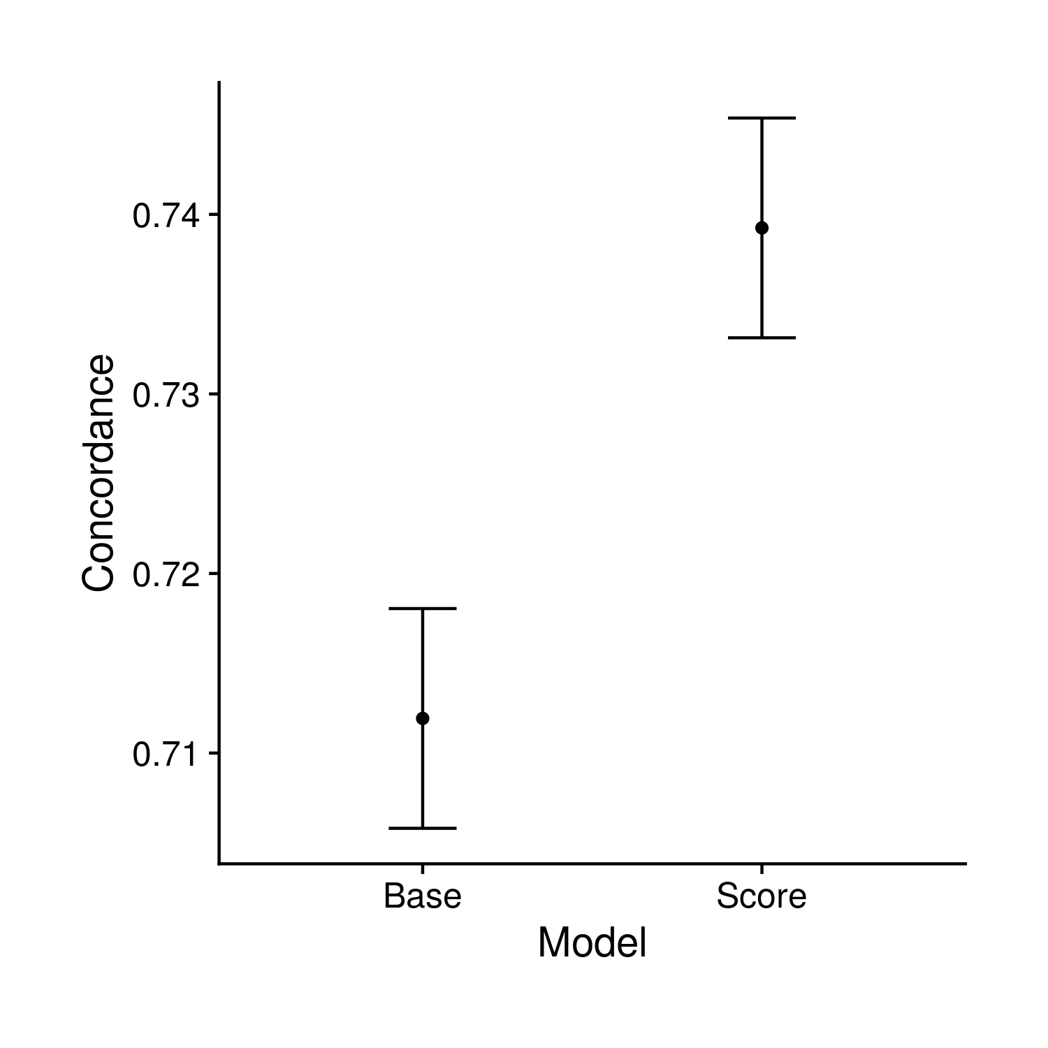
Figure 9.1: Testing comparison of concordance values

9.2.2 Survival Curve Fit

The second set of plots attempt to display the full set of fit survival curves. Previously in the tuning section this type of object could have breen created two ways. The first, fast way, by looking at people with average covariates other than the score which is given definite quantiles; the second, slow way, fits every single person individually and the averages together the survival curves for groups of people that fall in different polygenic risk score quantiles. To make things more accurate we now only use the slower method, and instead of just showing the final time point of the fit curves we show the full curve (along with the end time point). Specifically, the first two plots show these averaged curves for different polygenic risk score quantiles, the first with a standard error cone and the second comparing the base and score model generated curves. The final plot compared the base and score models at the final timepoint.

CODE GOES HERE

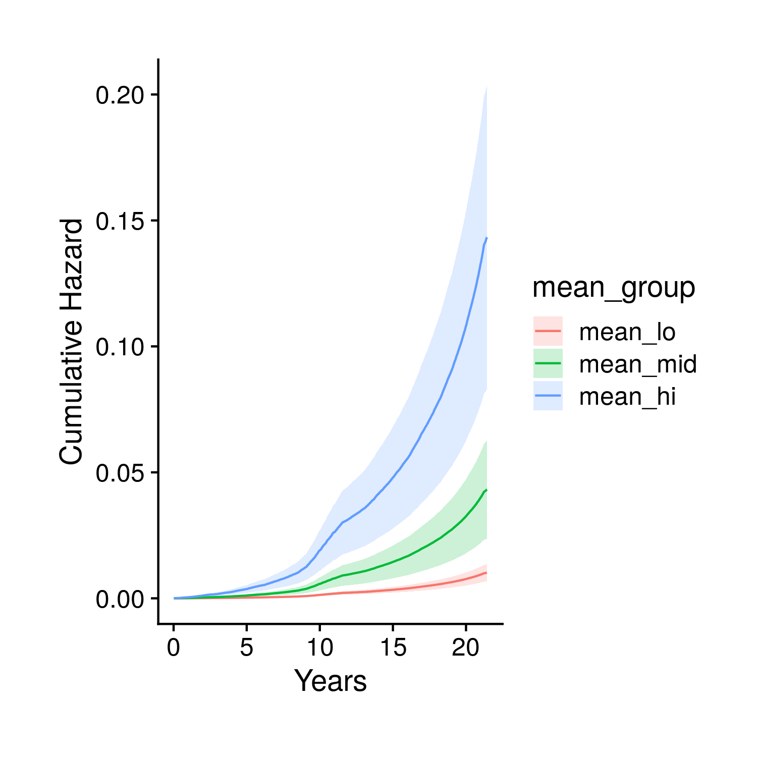
Figure 9.2: Kaplain-Meier style curve stratified by polygenic risk score quantiles

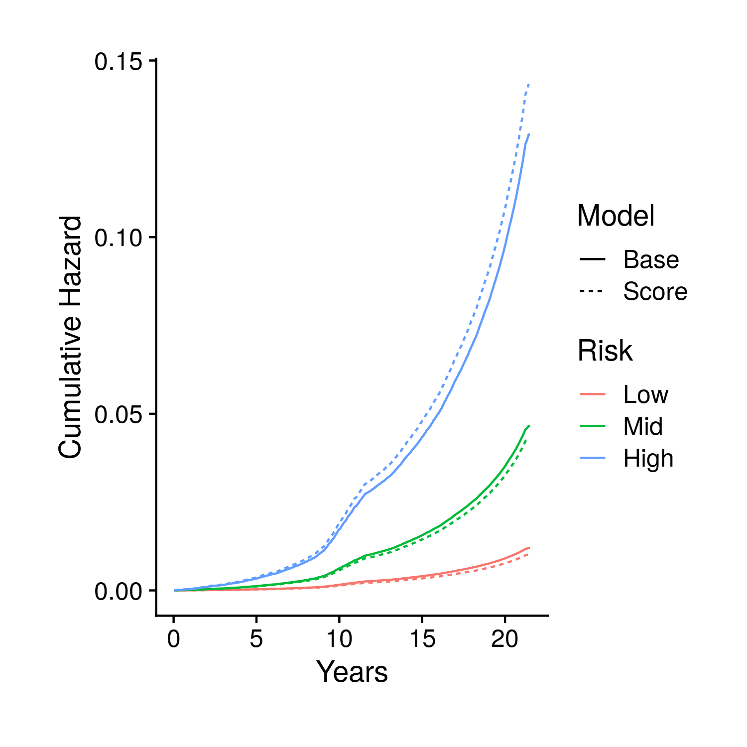
Figure 9.3: Kaplan-Meier style curves comparing groups stratified by polygenic risk score with two predictions, one that includes the score and one that does not, for each group

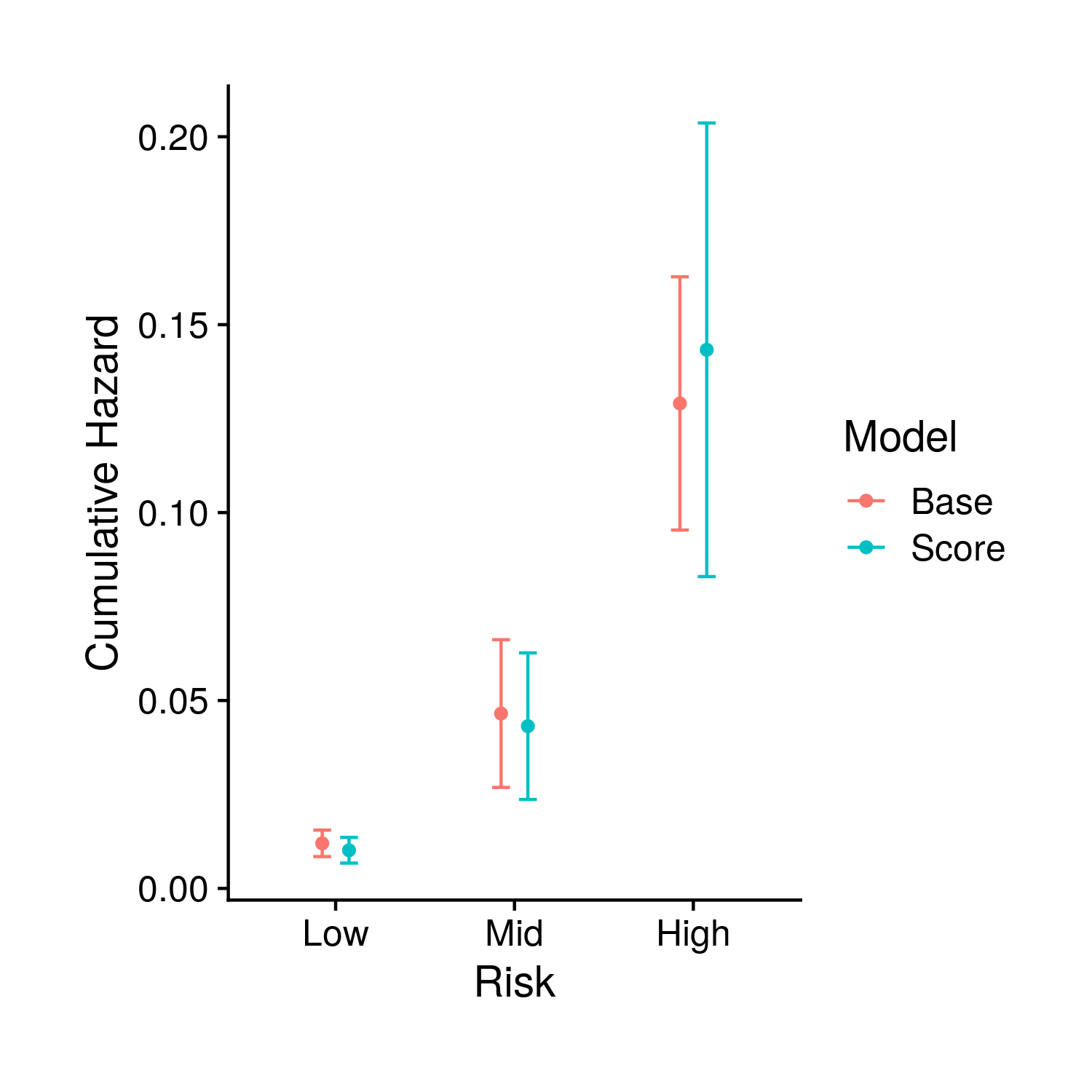
Figure 9.4: The estimed risk for the final time point in the previous plot, including confidence intervals

9.2.3 ROC and AUC

The plots derived from the ROC curve are very similar to concordance. The only difference is the addition of a plot that shows the ROC curves, comparing the score and base models.

CODE GOES HERE

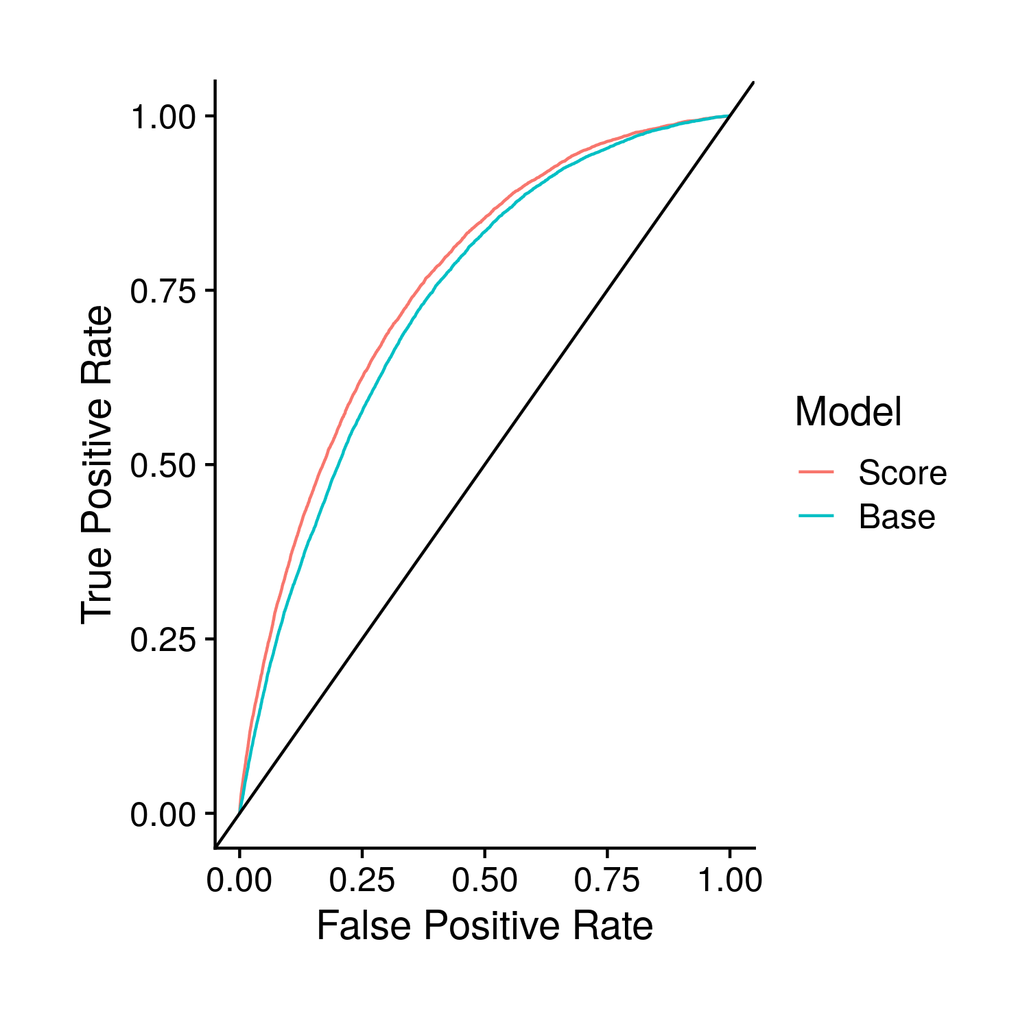
Figure 9.5: Comparison of the base and polygenic risk score included models through their ROC curves

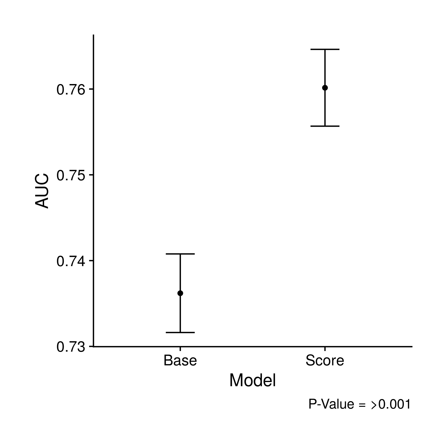
Figure 9.6: Comparison of the AUC values and their confidence intervals of the previous two ROC curves

9.2.4 Odds Ratios

In the same theme as the last few plots the single odds ratio plot compares the odds ratio from both the score and base models. This plot differs from the tuning as it includes multiple cut-off values, or points in which the respective model risk probability was cut to create an “exposed” and “non-exposed” group.

CODE GOES HERE

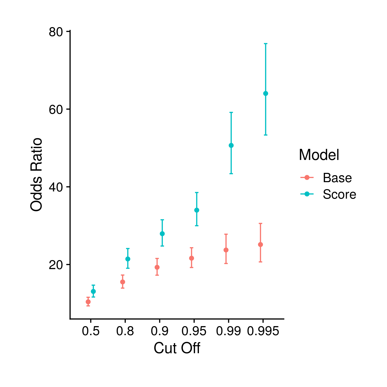
Figure 9.7: Comparison of odds ratios between the base and polygenic risk score included models

9.2.5 PR Curves

The plot for the PR Curves are completely novel relative to the tuning plots. However, the actual form of the plots is highly similar to the ROC plots, in the fact it compares the score and base model through curves. In this plot specifically the area under the PR curves is included as a caption.

CODE GOES HERE

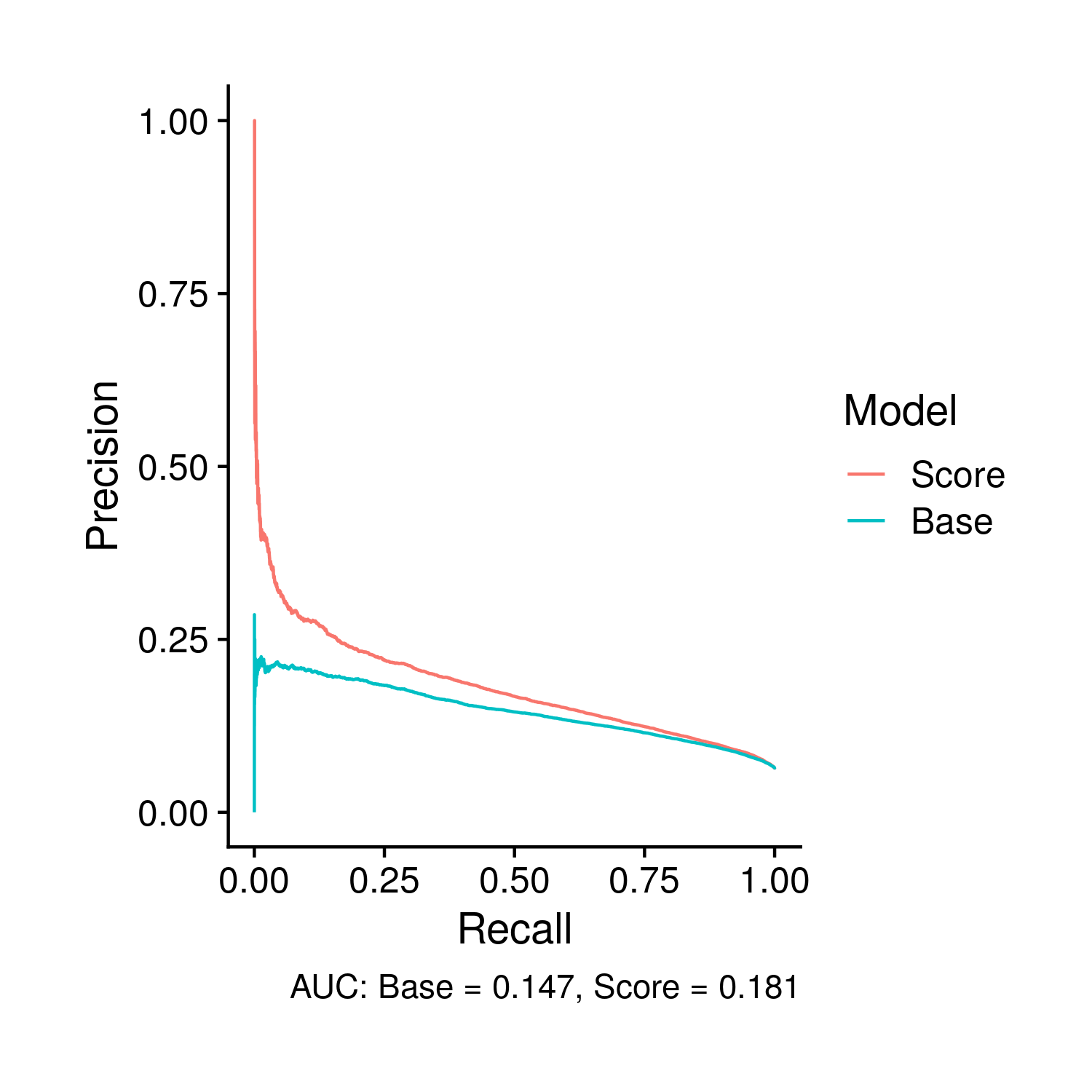
Figure 9.8: Comparison of the PR curves, and the area there under, between the base and polygenic risk score included models

9.2.6 Other Scores

While I have tried very hard to make the polygenic risk score so far analyzed to be the best polygenic risk score possible, there were countless decisions I have made in this process that could have been made differently by other researchers. To determine whether or not those other decisions would have been better I have downloaded the polygenic risk scores from PGS Catalog, analyzed them then plotted just the AUC comparison. I figure showing the other statistics would be largely redundant. The simple plot is:

CODE GOES HERE

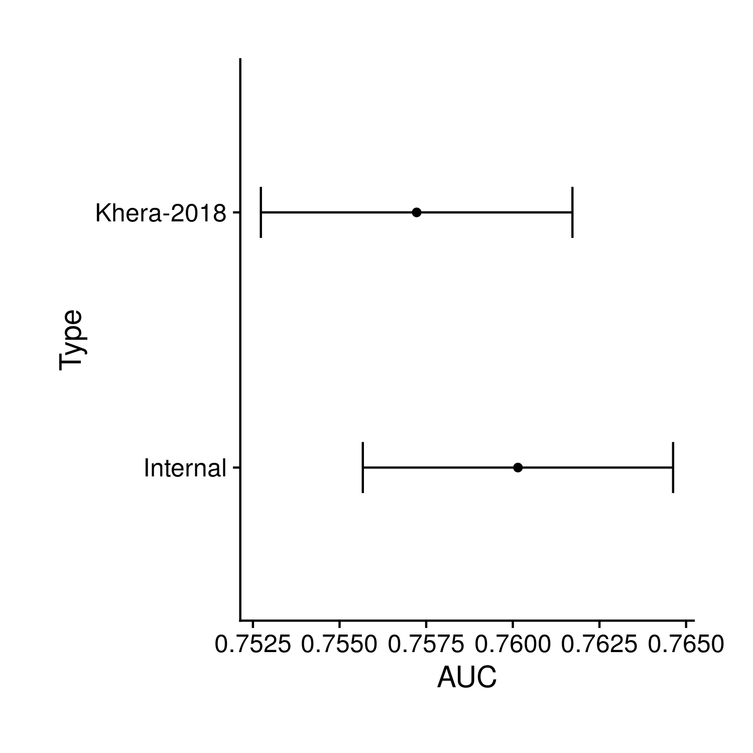
Figure 9.9: Comparison of the internal polygenic risk score analyzed so far and an externally prepared score (by other researchers)

9.2.7 Extra Covariates

Even though I have computed the effect of extra covariates within a model and their impact on odds ratio and PR, I have elected to only plot their effect on AUC. The thinkning is that the effect of the extra covariates will likely be the same across statistics so this is just a neater way. For my single AUC plot I am producing a figure that is very similar to the previous AUC plot although now there are colors to denote whether the model includes the extra covariates on top of the base covariates.

CODE GOES HERE

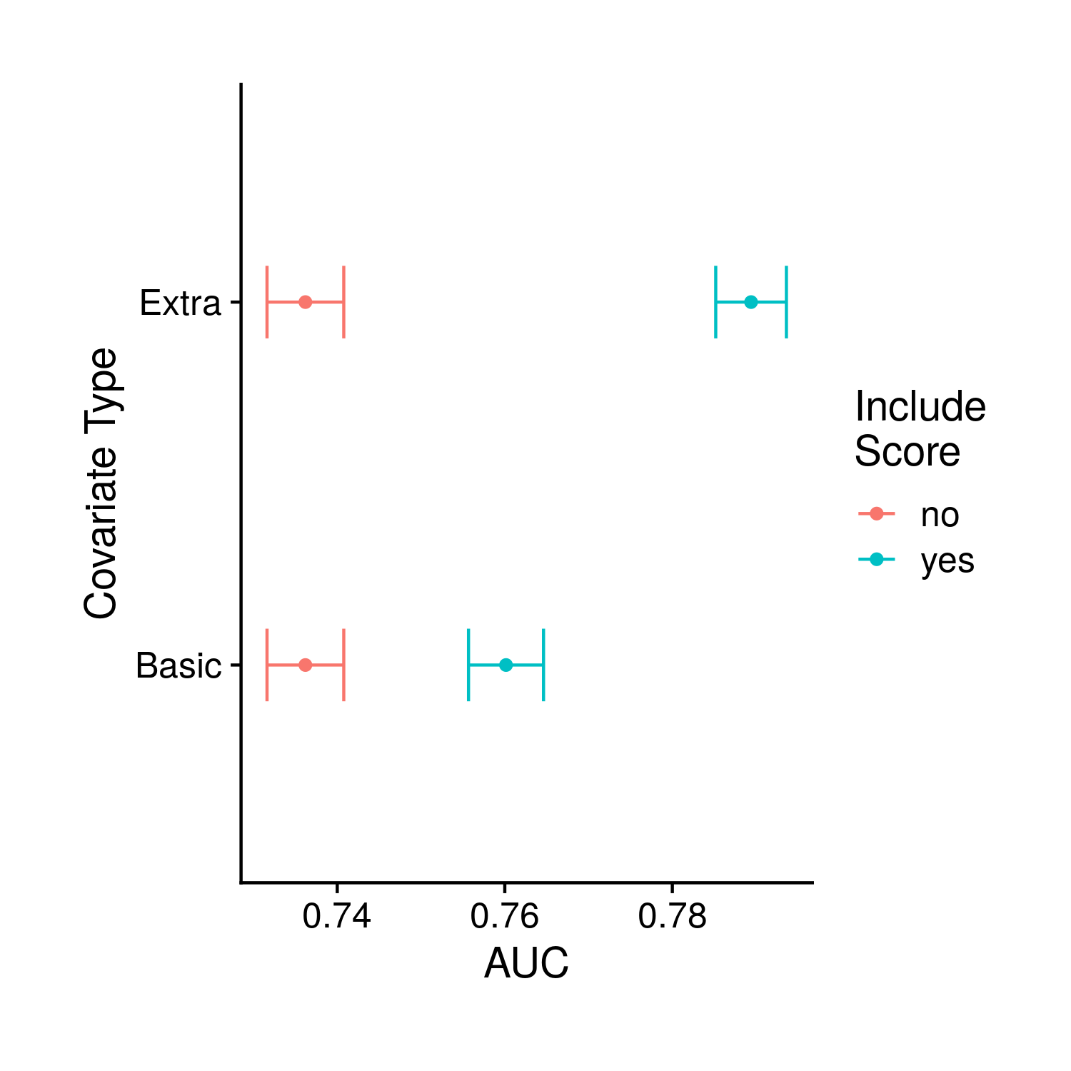
Figure 9.10: Comparison of the base model with and without the polygenic risk score, and with and without additional possible risk factors

9.2.8 Saving

The very last part of this process is saving all of the plots. Similar to tuning I leave the option to specify which plots one wants to save, but since we have already greatly reduced the number of plots under analysis saving everything does not seem like that large of a burden (and therefore saving everything is the default option).

CODE GOES HERE