11 Non-Predictive Evaluation
There are many facets of polygenic risk scores that are important in understanding if a score is best, that have nothing to do with its predictive value. These facets include the score size, the variation in response to phenotype definition, application differences in racial groups, and differences between sibling types. There are likely even more facets but these are the facets that I could think of and are likely the most critical and easy to do. Some of these sub-analyses require more than just a little R code, and I will go into the set-up in each respective section. Additional descriptions on what certain sub-analyses mean will also be in their respective sections. While these non-predictive evaluations may seem purely supplementary, I believe they are of paramount importance in truly understanding the quality of a polygenic risk score.
11.1 Individual Score Evaluation
I perform two major sets of evaluations, those that apply to each and every score (often in the effort of determining “model” fit and score qualities) and those that require multiple scores in order to establish comparisons (determine correlations between scores, parameters, meta-statistics). The first set of evaluations are of the former type.
11.1.1 Set Up
All of the nonpredictive evaluations are done within a single script, one author at a time. Before each of the previously mentioned evaluations can be carried out set up must be completed in which the scores and other nescessary files are read in. This set up is highly similar to what is done in the beginning of the tune script so I won’t go into much detail. The only major difference is that much of the code is duplicated (not a great practice but it works) so that the scores and remaining data for British individuals and non-British individuals are kept seperately. Remember that all of the other analyses are only done on a homogenous (mostly) British population, but here we want to check out what happens if it is not so homogenous. The script ultimately produces scores, phenotypes, dates and covariates. The details are shown below:
library(survival)
library(data.table)
library(pROC)
library(epitools)

author <- "Mahajan"
#author <- commandArgs(trailingOnly=TRUE)

#read in scores
all_scores <-  readRDS(paste0("../../do_score/final_scores/all_score.", tolower(author), ".RDS"))
score_eids <- read.table("~/athena/doc_score/do_score/all_specs/for_eid.fam", stringsAsFactors=F)

other_scores <- readRDS(paste0("~/athena/doc_score/do_score/ethnic_scoring/final_scores/all_score.", tolower(author), ".RDS"))
ethnic_eids <- read.table("~/athena/doc_score/qc/ethnic_eids", stringsAsFactors=F)

#normalize the scores
scores <- all_scores[,grepl(tolower(author), colnames(all_scores))]
scores <- scores[,apply(scores, 2, function(x) length(unique(x)) > 3)]
scores <- apply(scores, 2, function(x) (x-mean(x)) / (max(abs((x-mean(x)))) * 0.01) )
rm(all_scores)

escores <- other_scores[,grepl(tolower(author), colnames(other_scores))]
escores <- escores[,apply(escores, 2, function(x) length(unique(x)) > 3)]
escores <- apply(escores, 2, function(x) (x-mean(x)) / (max(abs((x-mean(x)))) * 0.01) )
rm(other_scores)

#read in phenotype and covars
pheno <- read.table(paste0("../construct_defs/pheno_defs/diag.", tolower(author), ".txt.gz"), stringsAsFactors=F)
dates <- read.table(paste0("../construct_defs/pheno_defs/time.", tolower(author), ".txt.gz"), stringsAsFactors=F)
covars <- readRDS("../get_covars/base_covars.RDS")

#sort the phenotypes
pheno_eids <- read.table("../construct_defs/eid.csv", header = T)
pheno_eids <- pheno_eids[order(pheno_eids[,1]),]
pheno_eids <- pheno_eids[-length(pheno_eids)]

#split covars
brit_covars <- covars[(covars[,1] %in% score_eids[,1]) & (covars[,1] %in% pheno_eids),]
brit_covars <- brit_covars[order(brit_covars[,1]),]

ethnic_covars <- covars[(covars[,1] %in% ethnic_eids[,1]) & (covars[,1] %in% pheno_eids),]
ethnic_covars <- ethnic_covars[order(ethnic_covars[,1]),]

#split pheno, dates
brit_pheno <- pheno[(pheno_eids %in% score_eids[,1]) & (pheno_eids %in% covars[,1]),]
brit_dates <- dates[(pheno_eids %in% score_eids[,1]) & (pheno_eids %in% covars[,1]),]
brit_pheno_eids <- pheno_eids[(pheno_eids %in% score_eids[,1]) & (pheno_eids %in% covars[,1])]

ethnic_pheno <- pheno[(pheno_eids %in% ethnic_eids[,1]) & (pheno_eids %in% covars[,1]),]
ethnic_dates <- dates[(pheno_eids %in% ethnic_eids[,1]) & (pheno_eids %in% covars[,1]),]
ethnic_pheno_eids <- pheno_eids[(pheno_eids %in% ethnic_eids[,1]) & (pheno_eids %in% covars[,1])]

#split scores
brit_scores <- scores[(score_eids[,1] %in% pheno_eids) & (score_eids[,1] %in% covars[,1]),]
brit_score_eids <- score_eids[(score_eids[,1] %in% pheno_eids) & (score_eids[,1] %in% covars[,1]),]

brit_scores <- brit_scores[order(brit_score_eids[,1]),]
brit_eid <- brit_score_eids[order(brit_score_eids[, 1]), 1]

ethnic_scores <- escores[(ethnic_eids[,1] %in% pheno_eids) & (ethnic_eids[,1] %in% covars[,1]),]
ethnic_score_eids <- ethnic_eids[(ethnic_eids[,1] %in% pheno_eids) & (ethnic_eids[,1] %in% covars[,1]),,drop=F]

ethnic_scores <- ethnic_scores[order(ethnic_score_eids[,1]),]
ethnic_eid <- ethnic_score_eids[order(ethnic_score_eids[, 1]), 1]

exit()
rm(scores)
rm(escores)

#get the british eids
brit_train <- read.table("../../qc/cv_files/train_eid.0.6.txt", stringsAsFactors=F)
brit_test <- read.table("../../qc/cv_files/test_eid.0.4.txt", stringsAsFactors=F)

#remove possible sex group
author_defs <- read.table("../descript_defs/author_defs", stringsAsFactors=F, header=T)
sex_group <- author_defs[author_defs[,1] == author, 3]

if(sex_group == "M"){
  all_sex <- read.table("all_sex", stringsAsFactors=F, sep=",", header=T)
  all_sex <- all_sex[all_sex[,1] %in% ethnic_eid,]
  all_sex <- all_sex[order(all_sex[,1])[rank(ethnic_eid)],]

  brit_scores <- brit_scores[brit_covars$sex == 1,]
  brit_eid <- brit_eid[brit_covars$sex == 1]
  brit_pheno <- brit_pheno[brit_covars$sex == 1,]
  brit_dates <- brit_dates[brit_covars$sex == 1,]
  brit_covars <- brit_covars[brit_covars$sex == 1,]

  ethnic_scores <- ethnic_scores[all_sex[,2] == 1,]
  ethnic_eid <- ethnic_eid[all_sex[,2] == 1]
  ethnic_pheno <- ethnic_pheno[all_sex[,2] == 1,]
  ethnic_dates <- ethnic_dates[all_sex[,2] == 1,]
  ethnic_covars <- ethnic_covars[all_sex[,2] == 1,]

}else if(sex_group == "F"){
  all_sex <- read.table("all_sex", stringsAsFactors=F, sep=",", header=T)
  all_sex <- all_sex[all_sex[,1] %in% ethnic_eid,]
  all_sex <- all_sex[order(all_sex[,1])[rank(ethnic_eid)],]

  brit_scores <- brit_scores[brit_covars$sex == 0,]
  brit_eid <- brit_eid[brit_covars$sex == 0]
  brit_pheno <- brit_pheno[brit_covars$sex == 0,]
  brit_dates <- brit_dates[brit_covars$sex == 0,]
  brit_covars <- brit_covars[brit_covars$sex == 0,]

  ethnic_scores <- ethnic_scores[all_sex[,2] == 0,]
  ethnic_eid <- ethnic_eid[all_sex[,2] == 0]
  ethnic_pheno <- ethnic_pheno[all_sex[,2] == 0,]
  ethnic_dates <- ethnic_dates[all_sex[,2] == 0,]
  ethnic_covars <- ethnic_covars[all_sex[,2] == 0,]
}
11.1.2 Analysis of Score Sizes
Once the set-up is complete the first major analysis entail the score sizes and distribution of effects. This outcomes of this analysis can be telling. If the scores contain many SNPs than the underlying disease architechture is likely highly polygenic, but if that score focuses on a few SNPs with high effect, than we know our previous assumption about polygenicity may be wrong. Therefore we must analyze not only the size but also the distribution of effects. Further sub-analyses that focus on a method, or parameter set within a method can be telling of future expected behavoir, perhaps even indicating the most likely method that should be applied to a disease not yet scored.
The code that carries out this analysis collects 4 important measures of a score to better understand it. First is simply the number of SNPs. Second are the deciles of the absolute effect. The third and fourth measures get more complicated, and involve a splitter function that seperates the score SNPs into 4 groups such that each have nearly the equivalent sum of their absolute effect. The third measure is then the size of each of these 4 groups. The fourth measure is the mean absolute effect of each of these 4 groups. The motivation behind splitting the SNPs into groups is to determine whether a few SNPs carry the vast majority of the weight across all SNPs and therefore could be used on their own. The exact code is shown below:
##############################################
########### SCORE SIZES ####################
##############################################

splitter <- function(values, N){
  inds = c(0, sapply(1:N, function(i) which.min(abs(cumsum(as.numeric(values)) - sum(as.numeric(values))/N*i))))
  dif = diff(inds)
  if(any(dif == 0)){
    dif[1] <- dif[1] - sum(dif == 0)
    dif[dif == 0] <- 1
  }

  re = rep(1:length(dif), times = dif)
  return(split(values, re))
}


all_equal_splits_len <- matrix(0, nrow = ncol(brit_scores), ncol = 4)
all_equal_splits_mean <- matrix(0, nrow = ncol(brit_scores), ncol = 4)
all_quantiles <- matrix(0, nrow = ncol(brit_scores), ncol = 10)
all_len <- rep(0, ncol(brit_scores))

for(i in 1:ncol(brit_scores)){
  score_name <- colnames(brit_scores)[i]
  split_name <- strsplit(score_name, ".", fixed = T)[[1]]
  score_files <- list.files(paste0("~/athena/doc_score/mod_sets/", author, "/"), glob2rx(paste0(split_name[1], "*", split_name[3], ".", split_name[2], ".ss")))
  score_list <- list()
  for(j in 1:length(score_files)){
    #score_list[[j]] <- read.table(paste0("~/athena/doc_score/mod_sets/", author, "/", score_files[j]), stringsAsFactors = F, header = F)
    score_list[[j]] <- as.data.frame(fread(paste0("~/athena/doc_score/mod_sets/", author, "/", score_files[j])))
    colnames(score_list[[j]]) <- c("CHR", "BP", "RSID", "A1",  "A2", "SE", "BETA", "P", "ESS")
  }

  ss <- do.call("rbind", score_list)
  ss <- ss[!is.na(ss[,7]),]
  if(ss[1,7] == "BETA"){
    ss <- ss[ss[,7] != "BETA",]
    ss[,7] <- as.numeric(ss[,7])
  }
  ss[,7] <- as.numeric(ss[,7])
  ss <- ss[!is.na(ss[,7]) & ss[,7] != 0,]
  ss$eff <- abs(ss[,7])
  ss <- ss[order(ss$eff),]

  if(nrow(ss) > 10){
    all_equal_splits_len[i,] <- unlist(lapply(splitter(ss$eff, 4), length))
    all_equal_splits_mean[i,] <- unlist(lapply(splitter(ss$eff, 4), mean))
  } else {
    all_equal_splits_len[i,] <- rep(NA, 4)
    all_equal_splits_mean[i,] <- rep(NA, 4)
  }
  if(nrow(ss) > 100){
    all_quantiles[i,] <- quantile(ss$eff, 1:10/10)
  } else {
    all_quantiles[i,] <- rep(NA, 10)
  }
  all_len[i] <- length(ss$eff)
}

return_score_sizes <- list("all_equal_splits_len" = all_equal_splits_len, "all_equal_splits_mean" = all_equal_splits_mean, "all_quantiles" = all_quantiles, "all_len" = all_len)
11.1.3 Analysis of Phenotype Definitions
The second major analysis slightly breaks the definition of a non-predictive evaluation, as this analysis computes the AUC of each score using multiple phenotype definitions. As a quick reminder, there are multiple places within the UK Biobank that may indicate a person has a disease. Within the main tuning section we assume that if either the ICD records contain or the individual self-reports as having the disease we assume that they do. However, we could instead look at just the ICD records, creating a different phenotype definition. In this analysis we look at six different phenotype definitions: ICD records only; self-reported only; ICD records or self-reported; ICD records, self-reported, OPCS records or associated medication; and the previous definition but two conditions are met instead of any. While a looser definition may have a grater number of individuals that did not truly have the disease, perhaps the increased sample size of true individuals will make up for it. This is the type of trade-off this analysis is attempting to examine.
To get a respective AUC value a logistic regression model is created with the covariates of age, sex, PC1-10 and the polygenic risk score. The model is then used to form a prediction on the testing set and placed within the ROC function. While this continual use of the testing set would be bad news if I was going to report the final AUC value as something that can be replicated, that is not what I am doing. These values are simply useful in a relative sense to one another. As a final note, I am also storing the number of cases in each phenotype definiton to compare which creates the largest sample size. The exact code is shown below:
##############################################
########### PHENOTYPE DEFINITIONS ####################
##############################################

icd_phen <- apply(brit_pheno[,3:4], 1, function(x) any(x==1))*1
selfrep_phen <- apply(brit_pheno[,1:2], 1, function(x) any(x==1))*1
diag_phen <- apply(brit_pheno[,1:5], 1, function(x) any(x==1))*1
any_phen <- apply(brit_pheno, 1, function(x) any(x==1))*1
double_phen <- apply(brit_pheno, 1, function(x) sum(x) > 1)*1
all_phens <- list(icd_phen, selfrep_phen, diag_phen, any_phen, double_phen)

all_phen_auc <- matrix(0, nrow = ncol(brit_scores), ncol = 15)
phen_type_starts <- seq(1, 15, 3)

for(i in 1:5){
  df <- data.frame(phen = all_phens[[i]], brit_covars)
  for(j in 1:ncol(brit_scores)){
    if(any(df$phen == 1)){
      df$score <- brit_scores[,j]
      train_df <- df[df$eid %in% brit_train[,1],]
      test_df <- df[df$eid %in% brit_test[,1],]
      mod <- glm(phen ~ age + sex + PC1 + PC2 + PC3 + PC4 + PC5 + PC6 + PC7 + PC8 + PC9 + PC10 + score, data = train_df, family = "binomial")
      test_roc <- roc(test_df$phen ~ predict(mod, test_df))
      all_phen_auc[j,(phen_type_starts[i]):(phen_type_starts[i]+2)] <- as.numeric(ci.auc(test_roc))
    } else {
      all_phen_auc[j,(phen_type_starts[i]):(phen_type_starts[i]+2)] <- c(NA, NA, NA)
    }
  }
}

return_pheno_defs <- list("all_phen_auc" = all_phen_auc, "total_phens" = unlist(lapply(all_phens, sum)))
11.1.4 Comparison Between the Sexes
In several publications concern has been raised on the idea that polygenic risk scores may work far better for males compared to females (or vice versa). Some people have even constructed scores specifically for either males or females in the hope that stratifying would raise accuracy. While I have clearly not done that here it may still be worthwhile to see if there is a large prediction difference. To compare I follow a procedure very similar to the phenotype comparison set up, in which I get the training data, seperate it between males and females, construct two models, form two predictions on the testing set and finally get 2 AUC values. The exact code is:
##############################################
########### SEX DIFFERENCES ####################
##############################################

diag_phen <- apply(brit_pheno[,1:5], 1, function(x) any(x==1))*1

if(sex_group == "A"){
  all_sex_auc <- matrix(0, nrow = ncol(brit_scores), ncol = 6)

  df <- data.frame(phen = diag_phen, brit_covars)
  sex_auc_p <- rep(NA, ncol(brit_scores))
  for(j in 1:ncol(brit_scores)){
    df$score <- brit_scores[,j]
    train_df <- df[df$eid %in% brit_train[,1],]
    test_df <- df[df$eid %in% brit_test[,1],]
    roc_holder <- list()
    for(sex in c(0,1)){
      sub_train_df <- train_df[train_df$sex == sex,]
      sub_test_df <- test_df[test_df$sex == sex,]
      sub_train_df <- sub_train_df[,-which(colnames(sub_train_df) == "sex")]
      sub_test_df <- sub_test_df[,-which(colnames(sub_test_df) == "sex")]
      mod <- glm(phen ~ age + PC1 + PC2 + PC3 + PC4 + PC5 + PC6 + PC7 + PC8 + PC9 + PC10 + score, data = sub_train_df, family = "binomial")
      test_roc <- roc(sub_test_df$phen ~ predict(mod, sub_test_df))
      all_sex_auc[j,(sex*3+1):(sex*3+3)] <- as.numeric(ci.auc(test_roc))
      roc_holder[[sex+1]] <- test_roc
    }
    sex_auc_p[j] <- roc.test(roc_holder[[1]], roc_holder[[2]], paired = FALSE)$p.value
  }
} else {
  all_sex_auc <- NULL
  sex_auc_p <- NULL
}

return_sex_split <- list("all_sex_auc" = all_sex_auc)
11.1.5 Comparison of Ethnic Groups
The third major analysis compares the score distributions of various ethnic groups. These ethnic groups were created by analyzing the PCA that was completed by the UK Biobank (described just below). The vast majority of the individuals are British, and used throughout the main tuning/testing, but now we look at other ethnic groups such as African, Asian and other European ancestry. Many other reports have shown that scores created on European summary statistics will be greatly skewed based on which ethnic group it is applied. There is an ongoing discussion on exactly why this is that I unfortunately don’t have time to go into here. My intentions are simply to see how bad this skew is in the scores I am making.
The process to determine ethnic groups was primarly carried out by reading in the 40 PCs calculated by the UK Biobank, then implementing K-means clustering (with a k of 3). Each cluster was then identified as belonging to a given ethnic group by merging with racial groups each individual self-identified with. Each k-means cluster was clearly one ethnic group, with only a handful of outliers. As a further precaution, individuals that were within the first percentile of being furthest from the center of their cluster center were removed. The remaining individuals were from that point onwards ascribed with the ethnicity of the cluster. The exact code that carried out this process is:
library(vroom)

# Column titles for the qc files
#19 = outliers in hetrozygosity
#20 = putative sex chromosome aneuploidy
#21 = in kinship table
#22 = excluded from kinship calcs
#23 = excess relatives
#24 = British ancestry
#25 = Used in PCA
#26 = PCs

#read in qc and the fam file, which contains the eids of the qc file
qc <- as.data.frame(vroom("../qc/ukb_sample_qc.txt", delim = " ", col_names = F))
fam <- read.table("../calls/ukbb.22.fam", stringsAsFactors = F)

#do brit thing
brit_fam <- fam[qc[,19] == 0 & qc[,20] == 0 & qc[,23] == 0 & qc[,24] == 1,]
brit_fam$eth <- 0
brit_fam$eth_name <- "brit"

#read in the phen
phen <- read.csv("../phenotypes/ukb26867.csv.gz", stringsAsFactors = F)

#subset according to the specified conditions within "Genetics of 38 blood and urine biomarkers in the UK Biobank"
good_fam <- fam[qc[,19] == 0 & qc[,20] == 0 & qc[,23] == 0,]

#subset the phen, qc, and fam files based on the good_fam above
phen$eid[is.na(phen$eid)] <- -999
phen <- phen[phen[,1] %in% good_fam[,1],]
qc <- qc[fam[,1] %in% phen[,1],]
fam <- fam[fam[,1] %in% phen[,1],]
phen <- phen[order(phen[,1])[rank(fam[,1])],]

#create vector for the survey answers of self-declared race
ethnic <- as.numeric(phen[,1288,drop=T])
ethnic_code <- rep(0, length(ethnic))
ethnic_code[ethnic %in% c(1, 1001, 1002, 1003)] <- 1 #european
ethnic_code[ethnic %in% c(4002, 4003, 4)] <- 2 #black
ethnic_code[ethnic %in% c(3, 5, 3001, 3002, 3003, 3004)] <- 3 #asian

#do the kmeans and then calculate distance of each eid to its respective center
euc_dist <- function(x1, x2) sqrt(sum((x1 - x2) ^ 2))
pcs <- qc[,26:65]
k_clu <- kmeans(pcs, 3)
#dist_to_center <- rep(0, length(ethnic_code))
#for(i in 1:3){
#  for(j in which(k_clu$cluster == i)){
#    dist_to_center[j] <- euc_dist(k_clu$centers[i,], pcs[j,])
#  }
#}
dist_to_center <- readRDS("dist_to_center.RDS")

#get the indices of the pca outliers
ancestry_remove <- list()
for(i in 1:3){
  cut_off <- quantile(dist_to_center[k_clu$cluster == i], 0.99)
  ancestry_remove[[i]] <- which(dist_to_center > cut_off & k_clu$cluster == i)
}

#Determine
all_sums <- c(sum(k_clu$cluster == 1),
              sum(k_clu$cluster == 2),
              sum(k_clu$cluster == 3))

#assign ethnic groups then kick out outliers
fam$eth_name <- ""
fam$eth_name[k_clu$cluster == which.max(all_sums)] <- "euro"
fam$eth_name[k_clu$cluster == which.min(all_sums)] <- "african"
fam$eth_name[k_clu$cluster == which(all_sums == sort(all_sums)[2])] <- "asian"
fam$eth <- 0
fam$eth[k_clu$cluster == which.max(all_sums)] <- 1
fam$eth[k_clu$cluster == which.min(all_sums)] <- 2
fam$eth[k_clu$cluster == which(all_sums == sort(all_sums)[2])] <- 3
fam <- fam[-unlist(ancestry_remove),]
phen <- phen[-unlist(ancestry_remove),]

#break out ancestry fams
euro_fam <- fam[fam$eth_name == "euro",]
african_fam <- fam[fam$eth_name == "african",]
asian_fam <- fam[fam$eth_name == "asian",]

#create special for not dead eids and not lost to follow up
bad_bool <- apply(phen[,which(colnames(phen) %in% c("X40000.0.0", "X191.0.0"))], 1, function(x) any(! (x == "")))
bad_eid <- phen$eid[bad_bool]
alive_fam <- fam[!(fam[,1] %in% bad_eid),]
alive_euro_fam <- euro_fam[!(euro_fam[,1] %in% bad_eid),]
alive_african_fam <- african_fam[!(african_fam[,1] %in% bad_eid),]
alive_asian_fam <- asian_fam[!(asian_fam[,1] %in% bad_eid),]

#specific country eids
england_eid <- phen$eid[!is.na(phen[,which(colnames(phen) == "X26410.0.0")])]
scotland_eid <- phen$eid[!is.na(phen[,which(colnames(phen) == "X26427.0.0")])]
wales_eid <- phen$eid[!is.na(phen[,which(colnames(phen) == "X26426.0.0")])]
alive_england_fam <- fam[!(fam[,1] %in% bad_eid) & (fam[,1] %in% england_eid),]
alive_scotland_fam <- fam[!(fam[,1] %in% bad_eid) & (fam[,1] %in% scotland_eid),]
alive_wales_fam <- fam[!(fam[,1] %in% bad_eid) & (fam[,1] %in% wales_eid),]


#write all of the tables
write.table(fam, "fam_files/qc_fam", row.names = F, col.names = F, quote = F, sep = '\t')
write.table(euro_fam, "fam_files/euro_fam", row.names = F, col.names = F, quote = F, sep = '\t')
write.table(african_fam, "fam_files/african_fam", row.names = F, col.names = F, quote = F, sep = '\t')
write.table(asian_fam, "fam_files/asian_fam", row.names = F, col.names = F, quote = F, sep = '\t')

write.table(alive_fam, "fam_files/qc_alive_fam", row.names = F, col.names = F, quote = F, sep = '\t')
write.table(alive_euro_fam, "fam_files/qc_alive_euro_fam", row.names = F, col.names = F, quote = F, sep = '\t')
write.table(alive_african_fam, "fam_files/qc_alive_african_fam", row.names = F, col.names = F, quote = F, sep = '\t')
write.table(alive_asian_fam, "fam_files/qc_alive_asian_fam", row.names = F, col.names = F, quote = F, sep = '\t')

write.table(alive_england_fam, "fam_files/qc_alive_england_fam", row.names = F, col.names = F, quote = F, sep = '\t')
write.table(alive_scotland_fam, "fam_files/qc_alive_scotland_fam", row.names = F, col.names = F, quote = F, sep = '\t')
write.table(alive_wales_fam, "fam_files/qc_alive_wales_fam", row.names = F, col.names = F, quote = F, sep = '\t')

write.table(brit_fam, "fam_files/brit_fam", row.names = F, col.names = F, quote = F, sep = '\t')
To characterize the score distribution within each ethnic group I simply calculate the mean, standard deviation, and quantiles for the respective distribution. I also compute basic T-tests between each of the ancestral samples. With the relatively massive sample sizes the p-values are very low, so to get a better idea of the magnitude of the diffrences I keep the t-statistic as well. This might get fancier later on but this is what I have right now. The code showing these calculations is below:
asian_fam <- read.table("~/athena/ukbiobank/custom_qc/fam_files/asian_fam", stringsAsFactors=F)
african_fam <- read.table("~/athena/ukbiobank/custom_qc/fam_files/african_fam", stringsAsFactors=F)
euro_fam <- read.table("~/athena/ukbiobank/custom_qc/fam_files/euro_fam", stringsAsFactors=F)

ethnic_scores <- as.data.frame(ethnic_scores)
ethnic_scores$ethnic <- "none"
ethnic_scores$ethnic[ethnic_eid %in% asian_fam[,1]] <- "asian"
ethnic_scores$ethnic[ethnic_eid %in% african_fam[,1]] <- "african"
ethnic_scores$ethnic[ethnic_eid %in% euro_fam[,1]] <- "euro"


brit_stats <- matrix(0, nrow = ncol(ethnic_scores)-1, ncol = 13)
euro_stats <- matrix(0, nrow = ncol(ethnic_scores)-1, ncol = 13)
african_stats <- matrix(0, nrow = ncol(ethnic_scores)-1, ncol = 13)
asian_stats <- matrix(0, nrow = ncol(ethnic_scores)-1, ncol = 13)

for(i in 1:(ncol(ethnic_scores)-1)){
  brit_ind <- which(colnames(brit_scores) == colnames(ethnic_scores)[1])
  brit_stats[i,] <- c(mean(brit_scores[,brit_ind]), sd(brit_scores[,brit_ind]), quantile(brit_scores[,brit_ind], 0:10/10))
  sub_score <- ethnic_scores[ethnic_scores$ethnic == "euro",i]
  euro_stats[i,] <- c(mean(sub_score), sd(sub_score), quantile(sub_score, 0:10/10))
  sub_score <- ethnic_scores[ethnic_scores$ethnic == "african",i]
  african_stats[i,] <- c(mean(sub_score), sd(sub_score), quantile(sub_score, 0:10/10))
  sub_score <- ethnic_scores[ethnic_scores$ethnic == "asian",i]
  asian_stats[i,] <- c(mean(sub_score), sd(sub_score), quantile(sub_score, 0:10/10))
}

tvals <- data.frame(matrix(NA, nrow = 6, ncol = ncol(ethnic_scores)-1))
for(i in 1:(ncol(ethnic_scores)-1)){
  brit_ind <- which(colnames(brit_scores) == colnames(ethnic_scores)[i])
  euro <- ethnic_scores[ethnic_scores$ethnic == "euro",i]
  african <- ethnic_scores[ethnic_scores$ethnic == "african",i]
  asian <- ethnic_scores[ethnic_scores$ethnic == "asian",i]
  brit <- brit_scores[,brit_ind]

  tvals[1,i] <- t.test(brit, euro)$stat
  tvals[2,i] <- t.test(brit, african)$stat
  tvals[3,i] <- t.test(brit, asian)$stat
  tvals[4,i] <- t.test(euro, asian)$stat
  tvals[5,i] <- t.test(euro, african)$stat
  tvals[6,i] <- t.test(african, asian)$stat
}

pvals <- data.frame(matrix(NA, nrow = 6, ncol = ncol(ethnic_scores)-1))
for(i in 1:(ncol(ethnic_scores)-1)){
  brit_ind <- which(colnames(brit_scores) == colnames(ethnic_scores)[i])
  euro <- ethnic_scores[ethnic_scores$ethnic == "euro",i]
  african <- ethnic_scores[ethnic_scores$ethnic == "african",i]
  asian <- ethnic_scores[ethnic_scores$ethnic == "asian",i]
  brit <- brit_scores[,brit_ind]

  pvals[1,i] <- t.test(brit, euro)$p.value
  pvals[2,i] <- t.test(brit, african)$p.value
  pvals[3,i] <- t.test(brit, asian)$p.value
  pvals[4,i] <- t.test(euro, asian)$p.value
  pvals[5,i] <- t.test(euro, african)$p.value
  pvals[6,i] <- t.test(african, asian)$p.value
}


return_ethnic_groups <- list("names_to_keep" = colnames(ethnic_scores), "brit_stats" = brit_stats, "euro_stats" = euro_stats, "african_stats" = african_stats, "asian_stats" = asian_stats)
11.1.6 Comparison of Siblings
This type of non-predictive evaluation was inspired by a paper entitled “Sibling validation of polygenic risk scores and complex trait prediction” by Lillen, Raben and Hsu. The main motivation with this idea is that polygenic risk scores may be easily confounded by family upbringing or other environmental effects. However, for siblings these effects are in the same direction and magnitude for both (or more) individuals, and therefore if one sibling gets a disease and the other does not we can conclude the environmental effects are likely not involved. Luckily for us the UK Biobank comes pre-packaged with person-to-person genetic relatedness files (just the same as the QC files). From this file we can extract siblings (I use the same definition as the paper I mentioned at the top).
The statistic used to examine polygenic risk scores and siblings is called the concordance. It’s easily calculated by taking all pairs of siblings in which one has the phenotype and the other does not. If the PGS of phenotype positive individual is greater than the other that pair is given the value of 1, otherwise they are assigned 0. The mean value of the vector of siblings’0’s and 1’s is the concordance. The higher the value the better our polygenic risk score is. We can repeat this exercise for non-siblings and compare the two concordances to see if the environmental effects are significant.
Computationally we complete this task with simple for loops and assigning the 1’s and 0’s to a vector. The exact code is shown below:
##############################################
########### SIBLING GROUPS ###################
##############################################

#have to look at sibling pairs compared to non-sibling pairs

sibs <- read.table("../get_covars/covar_data/sibs", stringsAsFactors=F, header=T)

use_pheno <- unname(apply(brit_pheno[,1:4], 1, function(x) 1 %in% x)*1)
df <- data.frame(pheno = use_pheno, brit_covars)

conc_ci <- function(conc, ss, cases){
  #see: The meaning and use of the area under a receiver operating characteristic (ROC) curve
  q1 <- conc/(2-conc)
  q2 <- (2*conc^2)/(1+conc)
  var <- ((conc*(1-conc) + (cases-1)*(q1-conc^2))+(ss-cases-1)*(q2-conc^2))/(cases*(ss-cases))
  c_logit <- log(conc/(1-conc))
  c_var_logit <- var/((conc*(1-conc))^2)
  ci_hi <- exp(c_logit+1.96*c_var_logit)/(1+exp(c_logit+1.96*c_var_logit))
  ci_lo <- exp(c_logit-1.96*c_var_logit)/(1+exp(c_logit-1.96*c_var_logit))
  return(matrix(c(ci_hi, ci_lo)))
}

all_sib_conc <- matrix(0, nrow = ncol(brit_scores), ncol = 6)
for(i in 1:ncol(brit_scores)){
  print(i)
  df$score <- brit_scores[,i]

  pheno_sibs <- sibs[sibs[,1] %in% df$eid[df$pheno == 1] | sibs[,2] %in% df$eid[df$pheno == 1],]
  pos_guess <- rep(NA, nrow(pheno_sibs))
  for(j in 1:nrow(pheno_sibs)){
    sub_df <- df[df$eid %in% pheno_sibs[j,],]
    if(nrow(sub_df) == 2){
      if(sum(sub_df$pheno) == 1){
        pos_guess[j] <- (sub_df$score[sub_df$pheno == 1] > sub_df$score[sub_df$pheno == 0])*1
      }
    }
  }

  pos_guess <- pos_guess[!is.na(pos_guess)]
  sib_conc <- sum(pos_guess)/length(pos_guess)
  if(sib_conc == 1){
    sib_conc_ci <- c(1,1)
  } else {
    sib_conc_ci <- as.numeric(conc_ci(sib_conc, length(pos_guess)*2, length(pos_guess)))
  }

  pos_guess <- rep(NA, nrow(pheno_sibs)*10)
  for(j in 1:length(pos_guess)){
    pos_guess[j] <- (df$score[sample(which(df$pheno == 1), 1)] > df$score[sample(which(df$pheno == 0), 1)])*1
  }

  nonsib_conc <- sum(pos_guess)/length(pos_guess)
  nonsib_conc_ci <- as.numeric(conc_ci(nonsib_conc, length(pos_guess)*2, length(pos_guess)))

  all_sib_conc[i,] <- c(sib_conc_ci[1], sib_conc, sib_conc_ci[2], nonsib_conc_ci[1], nonsib_conc, nonsib_conc_ci[2])
}


rownames(all_sib_conc) <- colnames(brit_scores)
colnames(all_sib_conc) <- c("sib_conc_ci_lo", "sib_conc", "sib_conc_ci_hi", "nonsib_conc_ci_lo", "nonsib_conc", "nonsib_conc_ci_hi")

return_sibling_groups <- list("all_sib_conc" = all_sib_conc)
11.1.7 Comparison of Age
The analyses described below were completed a fair amount of time after the original. Therefore, the code is not completely connected, as it comes from a different script. However, all of the variables/objects that are set-up will fulfill the requirements of these code snippets.
The first additional comparison of personal attributes involves age. In an attempt to make equal sized groups, similar to what was done in the sex comparison, an age was determined for each disease such that it split the cases (those with the disease) evenly. Also known as the median age of the cases. The following process followed very similarly to the sex difference analysis: splitting the sample into two and then fitting and assessing a model on each. The AUCs and the p-value representing the difference between the two underlying ROC curves are kept for analysis. The exact code is:
##############################################
########### AGE DIFFERENCE ####################
##############################################

split_age <- function(indf){
  quota <- sum(df$phen)/2
  age_cut <- min(indf$age)
  good_val <- sum(indf$phen[indf$age <= age_cut])
  while(good_val < quota){
    age_cut <- age_cut + 0.1
    good_val <- sum(indf$phen[indf$age <= age_cut])
  }
  indf$young_old <- 0
  indf$young_old[indf$age > age_cut] <- 1
  return(indf)
}

diag_phen <- apply(brit_pheno[,1:5], 1, function(x) any(x==1))*1

all_age_auc <- matrix(0, nrow = ncol(brit_scores), ncol = 6)

df <- data.frame(phen = diag_phen, brit_covars)
df <- split_age(df)
age_auc_p <- rep(NA, ncol(brit_scores))
for(j in 1:ncol(brit_scores)){
  df$score <- brit_scores[,j]
  train_df <- df[df$eid %in% brit_train[,1],]
  test_df <- df[df$eid %in% brit_test[,1],]
  roc_holder <- list()
  for(young in c(0,1)){
    sub_train_df <- train_df[train_df$young_old == young,]
    sub_test_df <- test_df[test_df$young_old == young,]
    sub_train_df <- sub_train_df[,-which(colnames(sub_train_df) == "young_old")]
    sub_test_df <- sub_test_df[,-which(colnames(sub_test_df) == "young_old")]
    if("sex" %in% colnames(sub_train_df)){
      mod <- glm(phen ~ age + sex + PC1 + PC2 + PC3 + PC4 + PC5 + PC6 + PC7 + PC8 + PC9 + PC10 + score, data = sub_train_df, family = "binomial")
    } else {
      mod <- glm(phen ~ age + PC1 + PC2 + PC3 + PC4 + PC5 + PC6 + PC7 + PC8 + PC9 + PC10 + score, data = sub_train_df, family = "binomial")
    }
    test_roc <- roc(sub_test_df$phen ~ predict(mod, sub_test_df))
    all_age_auc[j,(young*3+1):(young*3+3)] <- as.numeric(ci.auc(test_roc))
    roc_holder[[young+1]] <- test_roc
  }
  age_auc_p[j] <- roc.test(roc_holder[[1]], roc_holder[[2]], paired = FALSE)$p.value
}
11.1.8 Comparison of Many Other
Following-up on the age difference tests, I later on realized that it would be easy to test and valuable to learn how the performance splits for many other personal attributes. The process of splitting the entire testing sample and then fitting and assessing the seperate groups was completed in a simple loop. The real work therefore was not the modeling but selecting the variables and choosing proper splits. I chose four variables that were measured to the individual and hopefully well represent the social and environmental status of the individual. I similarly chose four variables that are measured through the census, reflecting the wider living arrangement of the individual. Similar to the age analysis, each of these eight variables were split with the goal of creating two equally sized groups. Once these splits were made just as before the models were fit and assessed. The exact code is shown below:
census_attrib <- read.table("census_attrib.txt", stringsAsFactors=F, header=T)
colnames(census_attrib) <- c("eid", "median_age", "unemployed", "very_good_health", "pop_dens")
survey_attrib <- read.table("survey_attrib.txt", stringsAsFactors=F, header=T, sep=",")
colnames(survey_attrib) <- c("eid", "time_address", "number_in_house", "income", "age_edu")
common_eid <- intersect(df$eid[df$eid %in% survey_attrib$eid], df$eid[df$eid %in% census_attrib$eid])


brit_scores <- brit_scores[df$eid %in% common_eid,]
df <- df[df$eid %in% common_eid,]
survey_attrib <- survey_attrib[survey_attrib$eid %in% common_eid,]
census_attrib <- census_attrib[census_attrib$eid %in% common_eid,]
survey_attrib <- survey_attrib[order(survey_attrib$eid)[rank(df$eid)],]
census_attrib <- census_attrib[order(census_attrib$eid)[rank(df$eid)],]
df <- cbind(df, survey_attrib[,-1], census_attrib[,-1])


#QC #################################
df$time_address[df$time_address < 0 & !is.na(df$time_address)] <- NA
df$bin_address <- NA
df$bin_address[df$time_address %in% 1:19 & !is.na(df$time_address)] <- 0
df$bin_address[df$time_address %in% 20:100 & !is.na(df$time_address)] <- 1

df$income[(df$income == -1 | df$income == -3) & !is.na(df$income)] <- NA
df$bin_income <- NA
df$bin_income[df$income %in% c(1,2) & !is.na(df$income)] <- 0
df$bin_income[df$income %in% c(3,4,5) & !is.na(df$income)] <- 1

df$number_in_house[(df$number_in_house == -1 | df$number_in_house == -3) & !is.na(df$number_in_house)] <- NA
df$number_in_house[df$number_in_house > 25 & !is.na(df$number_in_house)] <- NA
df$bin_in_house <- NA
df$bin_in_house[df$number_in_house %in% c(1,2) & !is.na(df$number_in_house)] <- 0
df$bin_in_house[df$number_in_house %in% 3:25 & !is.na(df$number_in_house)] <- 1

df$age_edu[df$age_edu < 0 & !is.na(df$age_edu)] <- NA
df$bin_edu <- NA
df$bin_edu[df$age_edu %in% 1:19 & !is.na(df$age_edu)] <- 0
df$bin_edu[df$age_edu %in% 20:40 & !is.na(df$age_edu)] <- 1

df$bin_census_age <- NA
df$bin_census_age[df$median_age > median(df$median_age, na.rm = T) & !is.na(df$median_age)] <- 0
df$bin_census_age[df$median_age <= median(df$median_age, na.rm = T) & !is.na(df$median_age)] <- 1

df$bin_census_employ <- NA
df$bin_census_employ[df$unemployed > median(df$unemployed, na.rm = T) & !is.na(df$unemployed)] <- 0
df$bin_census_employ[df$unemployed <= median(df$unemployed, na.rm = T) & !is.na(df$unemployed)] <- 1

df$bin_census_health <- NA
df$bin_census_health[df$very_good_health > median(df$very_good_health, na.rm = T) & !is.na(df$very_good_health)] <- 0
df$bin_census_health[df$very_good_health <= median(df$very_good_health, na.rm = T) & !is.na(df$very_good_health)] <- 1


df$bin_pop_den <- NA
df$bin_pop_den[df$pop_dens > median(df$pop_dens, na.rm = T) & !is.na(df$pop_dens)] <- 0
df$bin_pop_den[df$pop_dens <= median(df$pop_dens, na.rm = T) & !is.na(df$pop_dens)] <- 1
#####################################


vars_examine <- grep("bin", colnames(df), value=T)

for(j in 1:ncol(brit_scores)){
  df$score <- brit_scores[,j]
  train_df <- df[df$eid %in% brit_train[,1],]
  test_df <- df[df$eid %in% brit_test[,1],]

  for(var in vars_examine){
    for(bin_val in 0:1){

    sub_train_df <- train_df[train_df[var] == bin_val,]
    sub_test_df <- test_df[test_df[var]== bin_val,]

    if("sex" %in% colnames(sub_train_df)){
      mod <- glm(phen ~ age + sex + PC1 + PC2 + PC3 + PC4 + PC5 + PC6 + PC7 + PC8 + PC9 + PC10 + score, data = sub_train_df, family = "binomial")
    } else {
      mod <- glm(phen ~ age + PC1 + PC2 + PC3 + PC4 + PC5 + PC6 + PC7 + PC8 + PC9 + PC10 + score, data = sub_train_df, family = "binomial")
    }

    test_roc <- roc(sub_test_df$phen ~ predict(mod, sub_test_df))

    if(bin_val == 0){
      save_roc <- test_roc
    } else {
      all_pval[[which(vars_examine == var)]][j,1] <- roc.test(save_roc, test_roc)$p.value
    }
    all_auc[[which(vars_examine == var)]][j,(bin_val*3+1):(bin_val*3+3)] <- as.numeric(ci.auc(test_roc))

    }
  }
}
11.1.9 Plotting
The plotting process, which takes place locally compared to on the academic computing system, can be easily broken down into once section for each analysis conducted. However, before any of these sections can be carried out I first have to read in the data. I also read in the extra data that describes all of the score and method names. This small amount of code is:
library(stringr)
library(ggplot2)
library(cowplot)
library(reshape2)
library(viridis)
library(pROC)
theme_set(theme_cowplot())

author <- "Bentham"
all_authors <- unique(str_split(list.files("nonpred_results/per_score/"), fixed("."), simplify = T)[,1])
all_authors <- all_authors[-which(all_authors == "xie")]

for(author in all_authors){
  print(author)

nonpred_res <- readRDS(paste0("nonpred_results/per_score/", tolower(author), ".res.many.RDS"))
score_names <- nonpred_res[["extra"]][[1]]
method_names <- str_split(score_names, fixed("."), simplify = T)[,3]
best_in_method <- read.table(paste0("tune_results/", tolower(author), ".methods.ss"))

convert_names <- function(x, the_dict = method_dict){
  y <- rep(NA, length(x))
  for(i in 1:length(x)){
    if(x[i] %in% the_dict[,1]){
      y[i] <- the_dict[the_dict[,1] == x[i], 2]
    }
  }
  return(y)
}

method_dict <- read.table("local_info/method_names", stringsAsFactors = F)
disease_dict <- read.table("local_info/disease_names", stringsAsFactors = F, sep = "\t")

neat_method_names <- convert_names(method_names)
neat_score_names <- paste0(neat_method_names, "-", str_split(score_names, fixed("."), simplify = T)[,2])
Onto the first section: plotting of score sizes. This is the most complex section as many sub-analyses are involved. First I extract the simple score length component and plot all scores in detail and compiled together by method. this detailed and compiled by method pattern continues for the effect of equal length and equal splits mean effect. These plots are crowded as colors and symbols are invovled, but there is no other way I can think of to include that much information nicely. Lastly, I use a color gradient to depict all 10 deciles of absolute effects. Seeing as this plot is not saying much new and is quite confusing with the gradient I have elected not to save it.
#################################################################
##################### SCORE SIZES ###############################
#################################################################

#score sizes
score_size_res <- nonpred_res[["score_sizes"]]

all_len <- score_size_res[["all_len"]]
plot_df <- data.frame(neat_score_names, neat_method_names, all_len)
plot_df$neat_score_names <- factor(plot_df$neat_score_names, levels = plot_df$neat_score_names[order(plot_df$all_len)])

the_plot <- ggplot(plot_df, aes(all_len, neat_score_names, color = neat_method_names)) + geom_point() +
  labs(x = "Number SNPs in Score", y = "Score Names", color = "Method") +
  theme(axis.text.y = element_blank())
plot(the_plot)
ggsave(paste0("meta_plots/", tolower(author), ".nonpred.scoresize.1.png"),
       the_plot, "png", height=6, width=7)

mean_vals <- unlist(lapply(as.character(unique(plot_df$neat_method_names)), function(x) mean(plot_df$all_len[plot_df$neat_method_names == x])))
plot_df$neat_method_names <- factor(plot_df$neat_method_names, levels = as.character(unique(plot_df$neat_method_names))[order(mean_vals)])
the_plot <- ggplot(plot_df, aes(log10(all_len), neat_method_names)) + geom_boxplot() + geom_point() +
  labs(x = "log10(Number SNPs in Score)", y = "Method") +
  geom_hline(yintercept = 1:length(unique(plot_df$neat_method_names)) + 0.5, color = "grey80")
plot(the_plot)
ggsave(paste0("meta_plots/", tolower(author), ".nonpred.scoresize.2.png"),
       the_plot, "png", height=6, width=7)


saveRDS(plot_df, paste0("nonpred_results/derived_from_per_score/", author, ".score.len.RDS"))
###

#Equal Splits Mean
score_equal_splits_mean <- data.frame(score_size_res[["all_equal_splits_mean"]])
score_equal_splits_mean <- score_equal_splits_mean/rowSums(score_equal_splits_mean)
colnames(score_equal_splits_mean) <- c("Q1", "Q2", "Q3", "Q4")
score_equal_splits_mean$method <- neat_method_names
score_equal_splits_mean$score <- neat_score_names
save_labels <- score_equal_splits_mean$score[order(score_equal_splits_mean$Q1)]

score_equal_splits_mean <- melt(score_equal_splits_mean, id.vars = c("method", "score"))
score_equal_splits_mean$score <- factor(score_equal_splits_mean$score, levels = save_labels)
the_plot <- ggplot(score_equal_splits_mean, aes(value, score, shape = variable, color = method)) + geom_point() +
  labs(x = "Proportion of Mean Effect", y = "Score", color = "Quartile of\nAbs. Effect") +
  theme(axis.text.y = element_blank())
plot(the_plot)
ggsave(paste0("meta_plots/", tolower(author), ".nonpred.scoremean.1.png"),
       the_plot, "png", height=6, width=7)
saveRDS(score_equal_splits_mean, paste0("nonpred_results/derived_from_per_score/", author, ".score.mean_quant.RDS"))


the_plot <- ggplot(score_equal_splits_mean, aes(value, method, color = variable)) + geom_boxplot() +
  labs(x = "Proportion of Mean Effect", y = "Method", color = "Quartile") +
  geom_hline(yintercept = 1:length(unique(score_equal_splits_mean$method)) + 0.5, color = "grey80")
plot(the_plot)
ggsave(paste0("meta_plots/", tolower(author), ".nonpred.scoremean.2.png"),
       the_plot, "png", height=6, width=7)

###

#Equal Splits Len
score_equal_splits_len <- data.frame(score_size_res[["all_equal_splits_len"]])
score_equal_splits_len <- score_equal_splits_len/rowSums(score_equal_splits_len)
colnames(score_equal_splits_len) <- c("Q1", "Q2", "Q3", "Q4")
score_equal_splits_len$method <- neat_method_names
score_equal_splits_len$score <- neat_score_names
save_labels <- score_equal_splits_len$score[order(score_equal_splits_len$Q1)]

score_equal_splits_len <- melt(score_equal_splits_len, id.vars = c("method", "score"))
score_equal_splits_len$score <- factor(score_equal_splits_len$score, levels = save_labels)
the_plot <- ggplot(score_equal_splits_len, aes(value, score, shape = variable, color = method)) + geom_point() +
  labs(x = "Proportion of Length", y = "Score", color = "Quartile of\nAbs. Effect") +
  theme(axis.text.y = element_blank())
plot(the_plot)
ggsave(paste0("meta_plots/", tolower(author), ".nonpred.scoresplit.1.png"),
       the_plot, "png", height=6, width=7)
saveRDS(score_equal_splits_len, paste0("nonpred_results/derived_from_per_score/", author, ".score.len_quant.RDS"))

the_plot <- ggplot(score_equal_splits_len, aes(value, method, color = variable)) + geom_boxplot() +
  labs(x = "Proportion of Length", y = "Method", color = "Quartile") +
  geom_hline(yintercept = 1:length(unique(score_equal_splits_len$method)) + 0.5, color = "grey80")
plot(the_plot)
ggsave(paste0("meta_plots/", tolower(author), ".nonpred.scoresplit.2.png"),
       the_plot, "png", height=6, width=7)

###

#Quantiles
score_quantiles <- data.frame(score_size_res[["all_quantiles"]])
score_quantiles <- score_quantiles/rowSums(score_quantiles)
colnames(score_quantiles) <- paste0("Q.", 1:10)
score_quantiles$method <- neat_method_names
score_quantiles$score <- neat_score_names
score_quantiles$names <- score_names
save_labels <- score_quantiles$names[order(score_quantiles$Q.1)]

score_quantiles <- melt(score_quantiles, id.vars = c("method", "score", "names"))
score_quantiles$names <- factor(score_quantiles$names, levels = save_labels)
score_quantiles$Q <- as.numeric(str_split(score_quantiles$variable, fixed("."), simplify = T)[,2])
the_plot <- ggplot(score_quantiles, aes(value, names, color = Q)) + geom_point() +
  scale_y_discrete(labels = neat_method_names) +
  labs(x = "Proportion of Abs. Effect", y = "Method", color = "Quantile") +
  theme(axis.text=element_text(size=8)) +
  scale_color_viridis()
plot(the_plot)
Then the output plots look like:
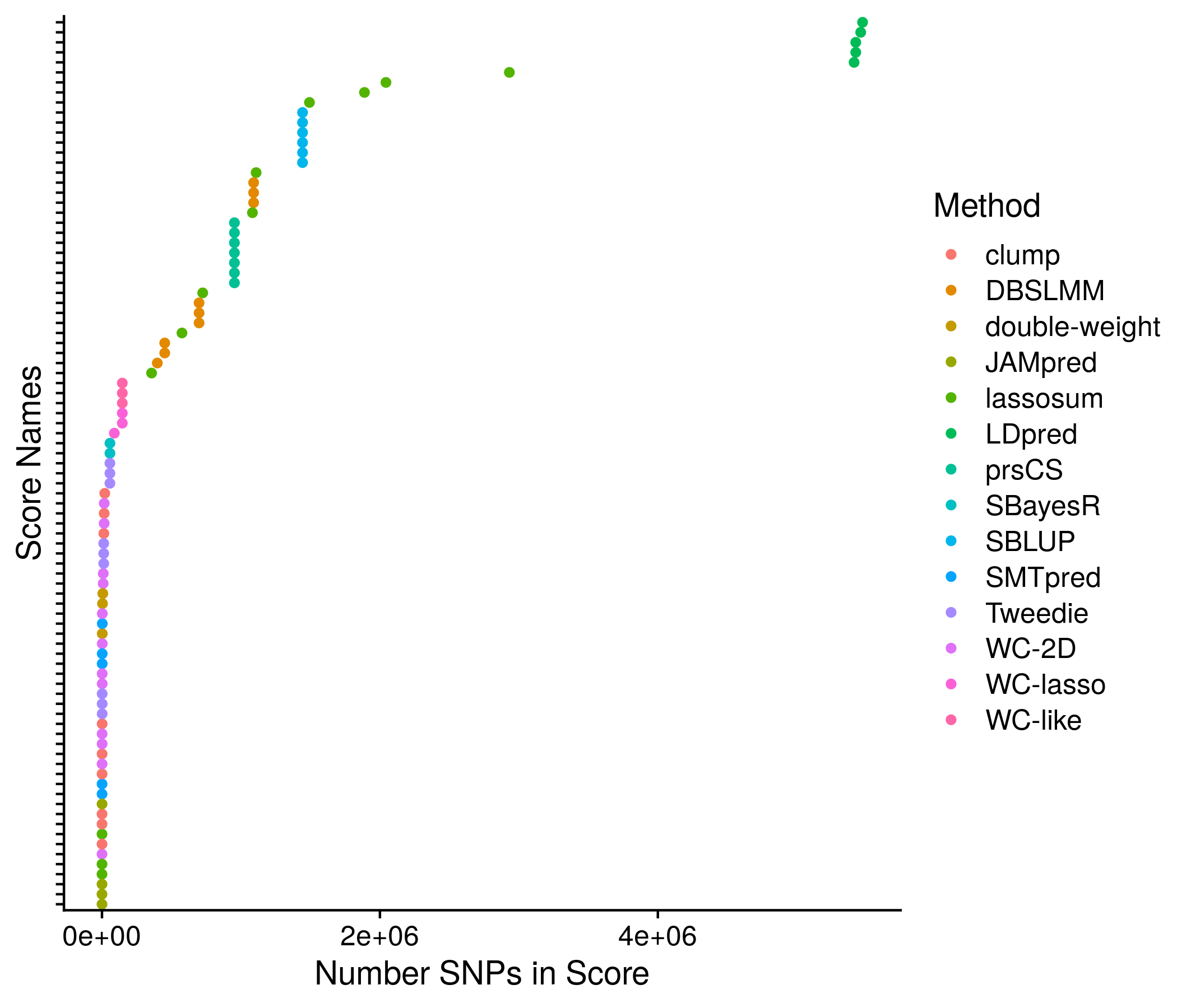
Figure 11.1: Example plot of the score sizes
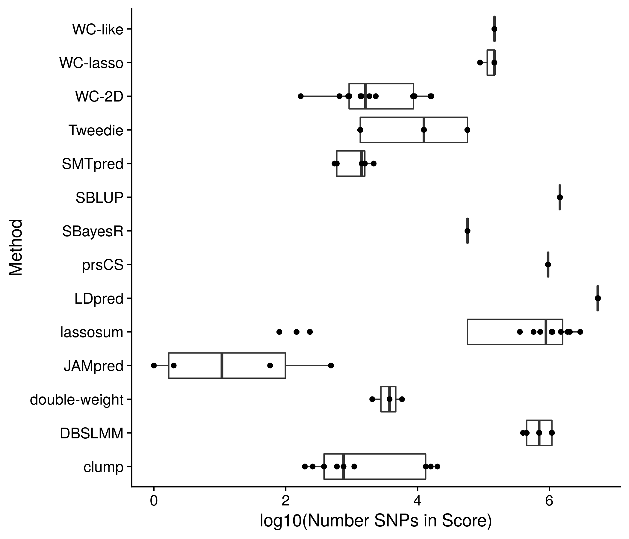
Figure 11.2: Another example plot of the score sizes
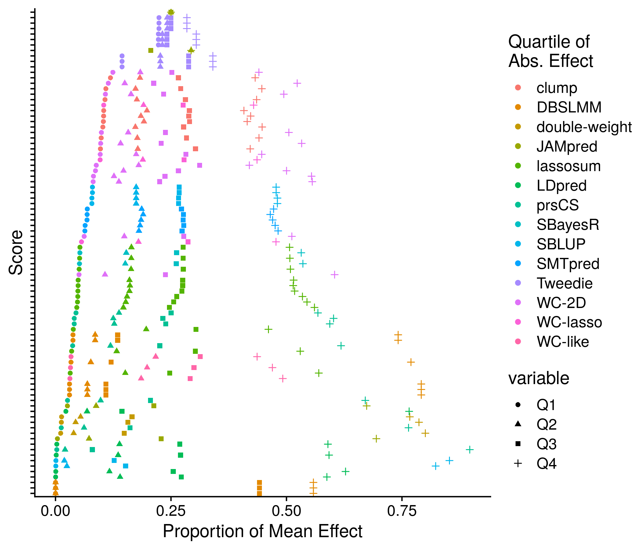
Figure 11.3: Example plot of the score means
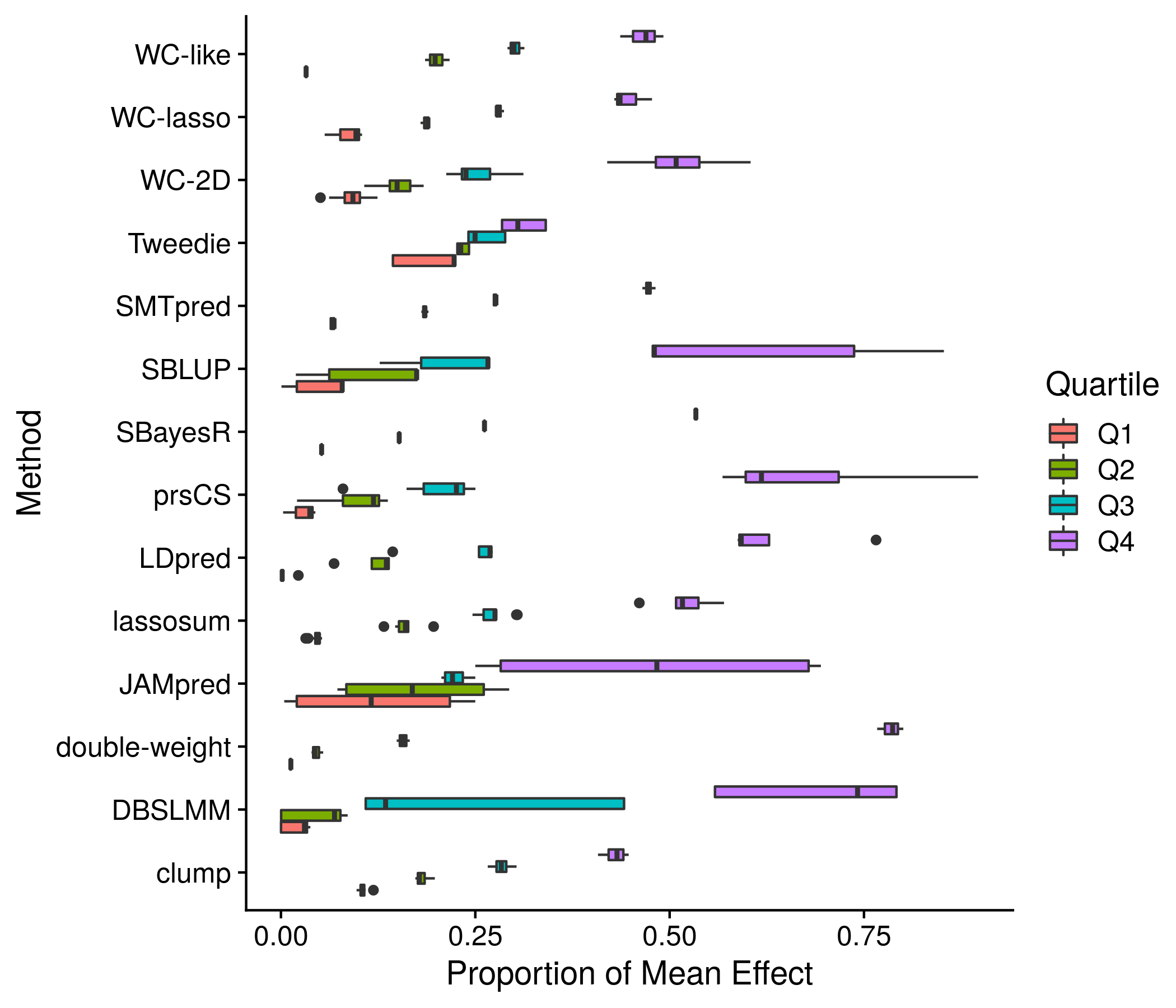
Figure 11.4: Another example plot of the score means
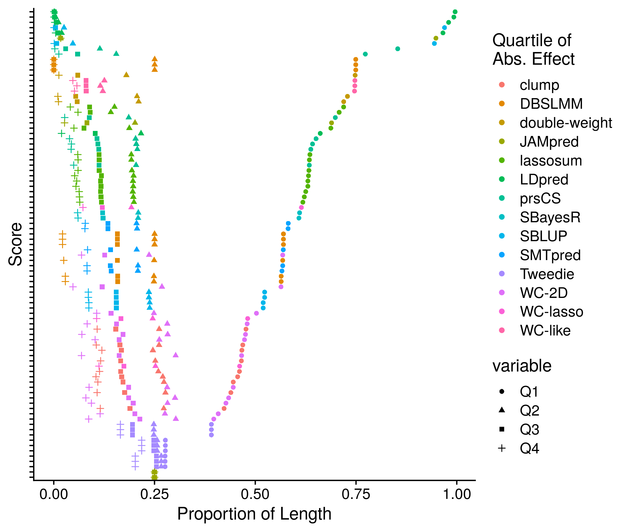
Figure 11.5: Example plot of the equal score splits by effect
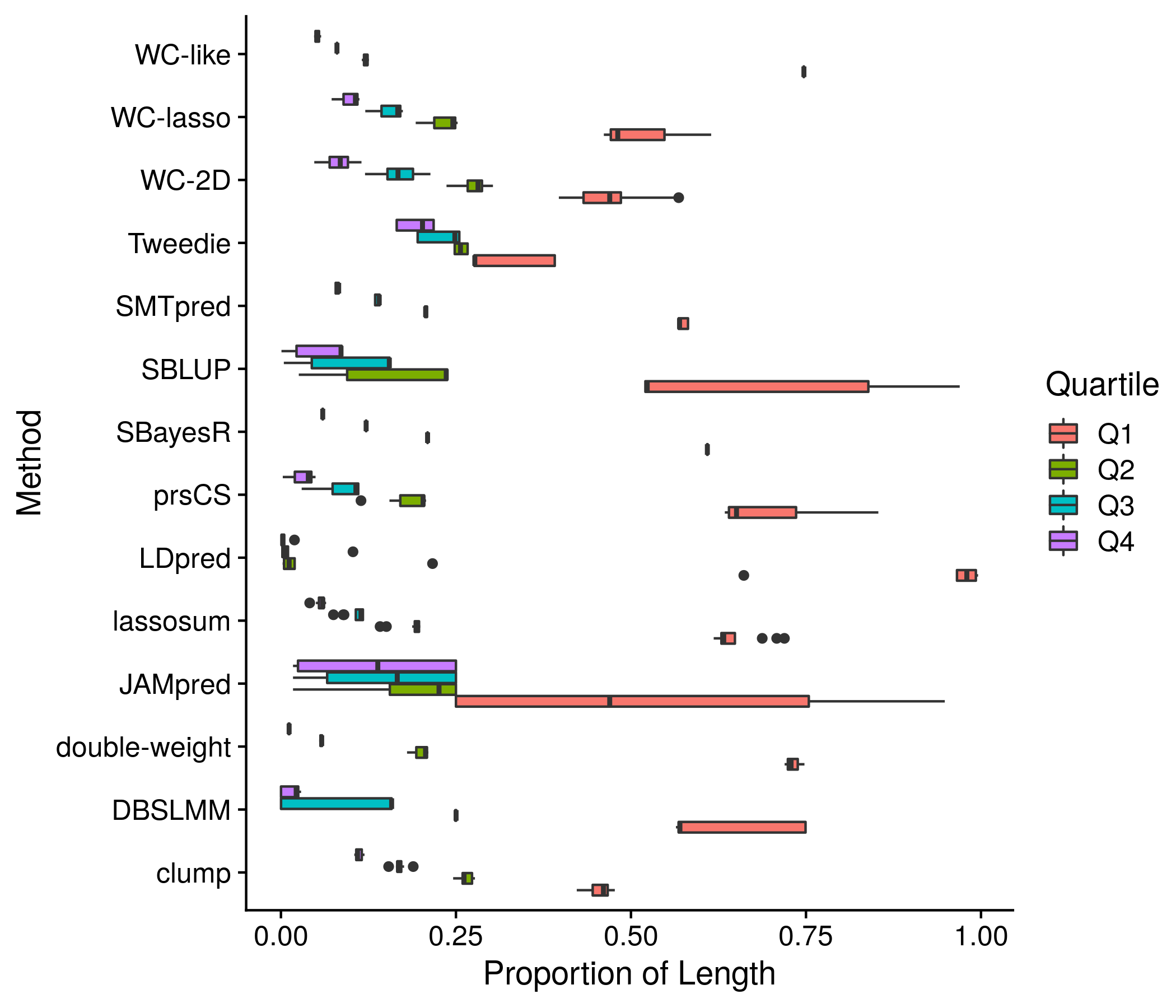
Figure 11.6: Example plot of the equal score splits by length
The next section: phenotype method. First I make a quick refrence plot of the number of cases for each method and phenotype. Next I show the AUC for each method, colored by the disease through both a series of boxplots and a heatmap. Showing the individual score detail seemed impossible/not useful so I did not attempt it, and rather grouped the scores together in the case of the boxplot and only kept the best AUC for each method in the case of the heatmap.
#################################################################
##################### PHENO DEFS ###############################
#################################################################

pheno_def_res <- nonpred_res[["pheno_defs"]]

#Cases
pheno_def_size <- as.data.frame(pheno_def_res[["total_phens"]])
colnames(pheno_def_size) <- "size"
pheno_def_size$method <- c("ICD", "Self\nReported", "ICD or\nSelf Rep.", "Any", "Double\nReported")
pheno_def_size$method <- factor(pheno_def_size$method, levels = pheno_def_size$method[order(pheno_def_size$size)])
the_plot <- ggplot(pheno_def_size, aes(size, method)) + geom_point() +
  labs(x = "Cases", y = "Phenotyping Method")
saveRDS(pheno_def_size, paste0("nonpred_results/derived_from_per_score/", author, ".pheno_def.len.RDS"))
plot(the_plot)
ggsave(paste0("meta_plots/", tolower(author), ".nonpred.phenodefs.1.png"),
       the_plot, "png", height=6, width=7)

#AUC
pheno_def_auc <- as.data.frame(pheno_def_res[["all_phen_auc"]])
pheno_def_auc <- pheno_def_auc[,seq(2,14,3)]
colnames(pheno_def_auc) <- c("ICD", "Self\nReported", "ICD or\nSelf Rep.", "Any", "Double\nReported")
pheno_def_auc$score <- neat_score_names
pheno_def_auc$method <- neat_method_names

# keep_score_names <- rep("", length(unique(neat_method_names)))
# for(m in unique(neat_method_names)){
#   keep_score_names[which(unique(neat_method_names) == m)] <- pheno_def_auc$score[pheno_def_auc$method == m][
#     which.max(pheno_def_auc$`ICD or\nSelf Rep.`[pheno_def_auc$method == m])]
# }
temp_save <- data.frame(pheno_def_auc)
pheno_def_auc <- melt(pheno_def_auc, id.vars = c("score", "method"))

mean_vals <- unlist(lapply(unique(pheno_def_auc$method),
                           function(x) mean(pheno_def_auc$value[pheno_def_auc$method == x & pheno_def_auc$variable == "ICD or\nSelf Rep."])))
pheno_def_auc$method <- factor(pheno_def_auc$method, levels = unique(pheno_def_auc$method)[order(mean_vals)])
the_plot <- ggplot(pheno_def_auc, aes(value, method, color = variable)) + geom_boxplot() +
  labs(x = "AUC", y = "Method", color = "Phenotyping\nMethod") +
  geom_hline(yintercept = 1:length(unique(pheno_def_auc$method)) + 0.5, color = "grey80")
plot(the_plot)
ggsave(paste0("meta_plots/", tolower(author), ".nonpred.phenodefs.2.png"),
       the_plot, "png", height=6, width=7)


pheno_def_auc <- temp_save[score_names %in% best_in_method[,1],]
pheno_def_auc <- melt(pheno_def_auc, id.vars = c("score", "method"))
the_plot <- ggplot(pheno_def_auc, aes(variable, method, fill = value)) + geom_raster() + scale_fill_viridis() +
  labs(x = "Phenotyping Method", y = "Method", fill = "AUC") +
  theme(axis.text.x = element_text(angle = 45, vjust = 1, hjust=1))
plot(the_plot)
ggsave(paste0("meta_plots/", tolower(author), ".nonpred.phenodefs.3.png"),
       the_plot, "png", height=6, width=7)
saveRDS(pheno_def_auc, paste0("nonpred_results/derived_from_per_score/", author, ".pheno_def.auc.RDS"))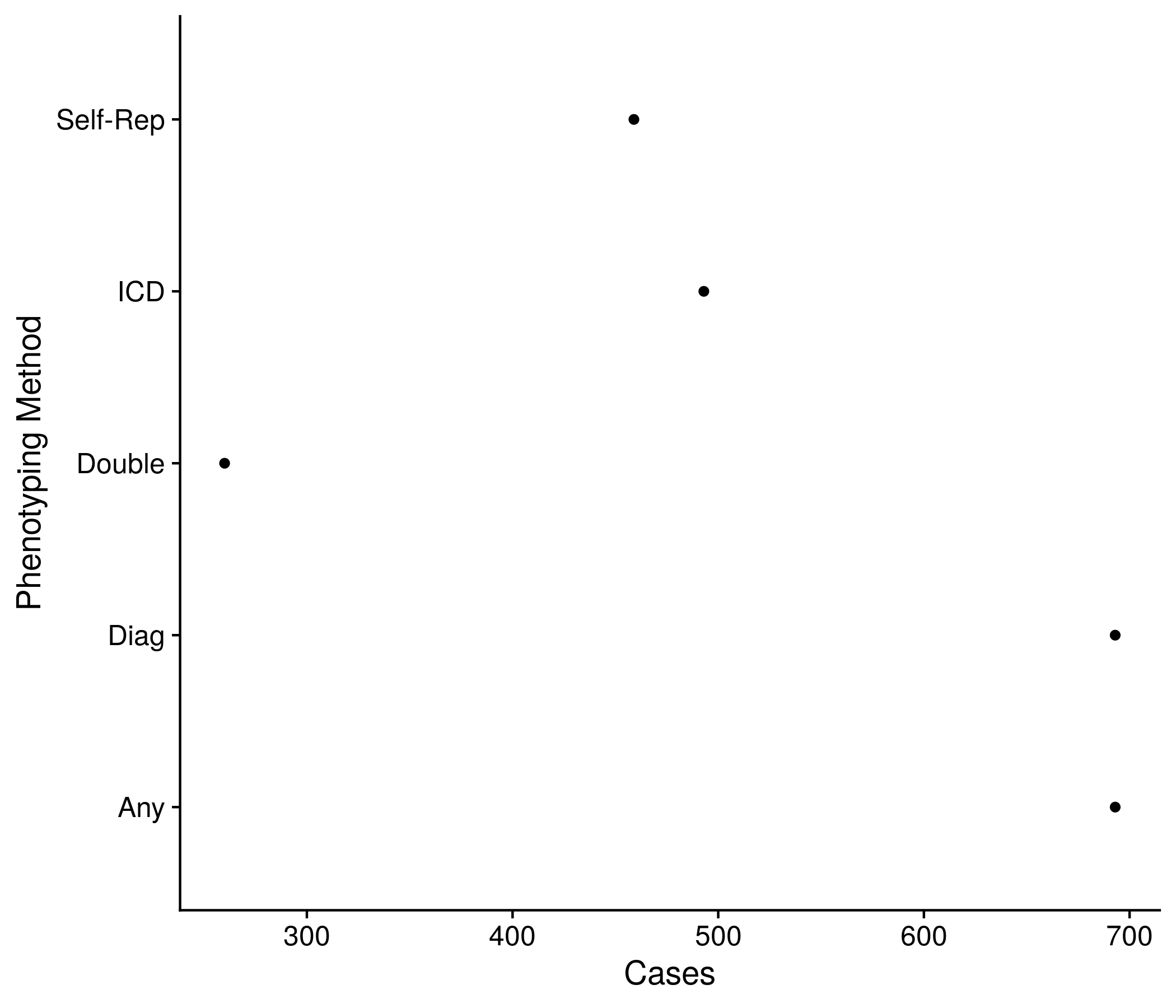
Figure 11.7: Example plot showing the number of cases by each method
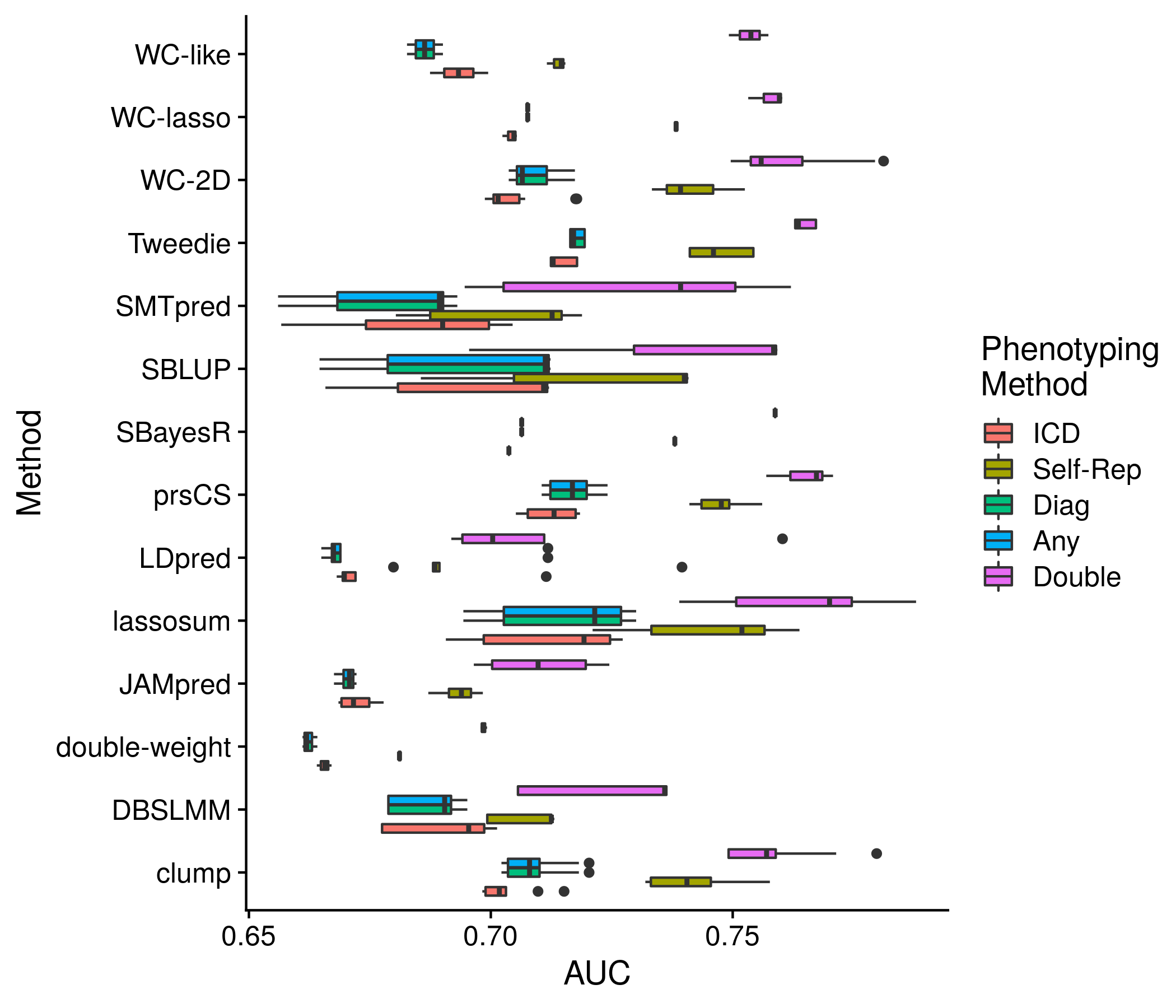
Figure 11.8: Example plot of the performance of each method (for all scores) by phenotype method
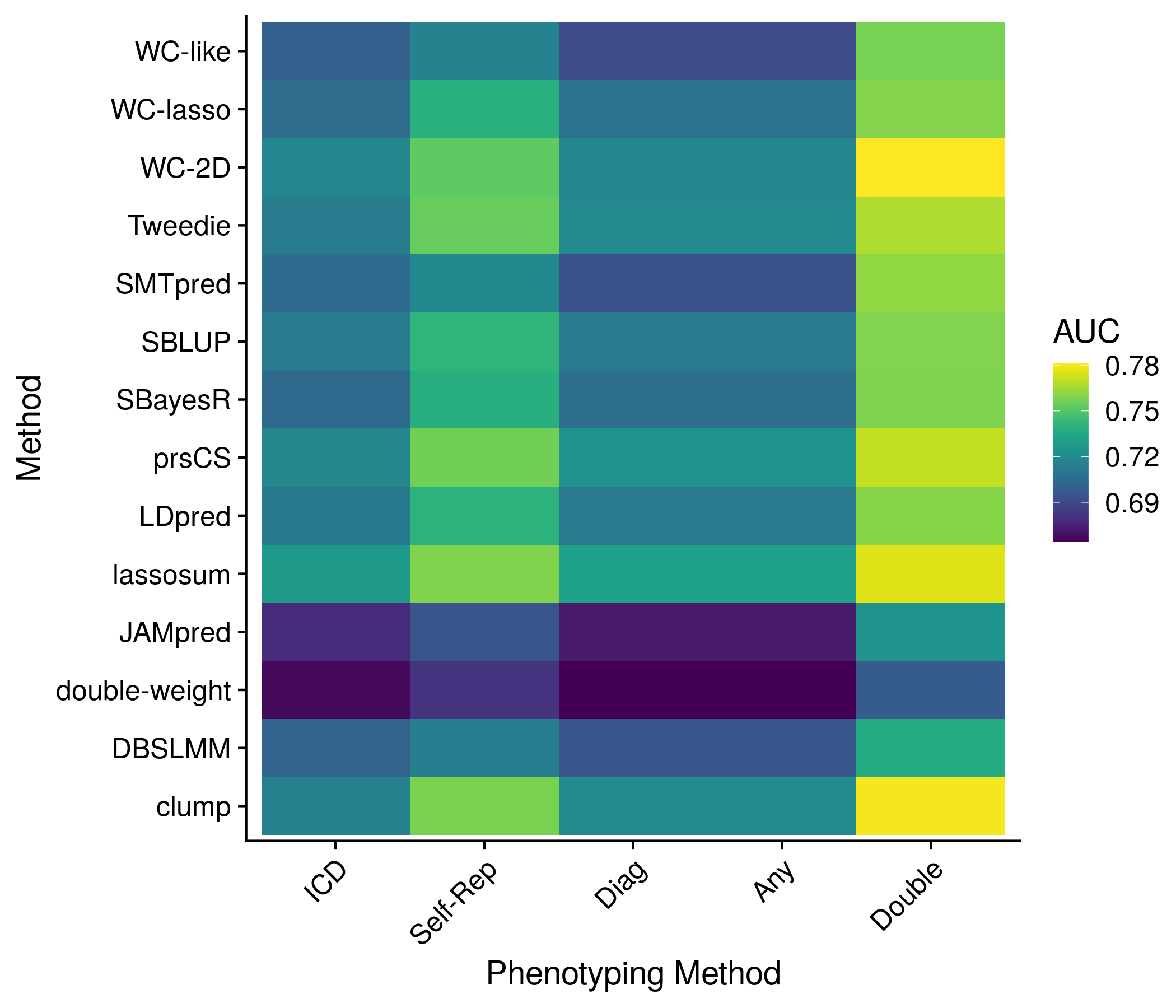
Figure 11.9: Example plot of the performance of each method (for the best score) by phenotype method
The next section: sex diffreences. Almost identical to the previous section I do not attempt to show every score and instead group the scores for each method in a series of boxplots, or look at just the best score for each method, however this time plotting the AUC with CIs for male and female.
#################################################################
##################### SEX DIFF ###############################
#################################################################

if(!is.null(nonpred_res[["sex_split"]][[1]])){
    sex_res <- as.data.frame(nonpred_res[["sex_split"]][[1]])

    # keep_score_names <- rep("", length(unique(neat_method_names)))
    # for(m in unique(neat_method_names)){
    #   keep_score_names[which(unique(neat_method_names) == m)] <-
    #     neat_score_names[neat_method_names == m][which.max(sex_res[neat_method_names == m,2])]
    # }

    colnames(sex_res) <- c("female_lo", "female_auc", "female_hi", "male_lo", "male_auc", "male_hi")
    sex_res$score_name <- neat_score_names
    sex_res$methods_name <- neat_method_names
    temp_save <- data.frame(sex_res)

    plot_df <- melt(sex_res, id.vars = c("score_name", "methods_name"))
    plot_df <- plot_df[plot_df$variable %in% c("female_auc", "male_auc"),]

    mean_vals <- unlist(lapply(unique(plot_df$methods_name), function(x) mean(plot_df$value[plot_df$methods_name == x])))
    plot_df$methods_name <- factor(plot_df$methods_name, levels = unique(plot_df$methods_name)[order(mean_vals)])
    the_plot <- ggplot(plot_df, aes(value, methods_name, color = variable)) + geom_boxplot() +
      labs(x = "AUC", y = "Methods", color = "Sex") +
      scale_color_discrete(labels = c("Female", "Male")) +
      geom_hline(yintercept = 1:length(unique(plot_df$methods_name)) + 0.5, color = "grey80")
    plot(the_plot)
    ggsave(paste0("meta_plots/", tolower(author), ".nonpred.sexdiff.1.png"),
           the_plot, "png", height=6, width=7)

    plot_df <- temp_save
    plot_df <- sex_res[,c(1:3,7,8)]
    colnames(plot_df) <- c("male_lo", "male_auc", "male_hi", "score_name", "methods_name")
    plot_df <- rbind(plot_df, temp_save[,4:8])
    plot_df$sex <- c(rep("female", nrow(sex_res)), rep("male", nrow(sex_res)))

    plot_df <- plot_df[score_names %in% best_in_method[,1],]
    plot_df$sex <- str_to_title(plot_df$sex)
    plot_df$methods_name <- factor(plot_df$methods_name, levels =
                                     plot_df$methods_name[plot_df$sex == "Male"][order(plot_df$male_auc[plot_df$sex == "Male"])])

    the_plot <- ggplot(plot_df, aes(male_auc, methods_name, color = sex)) +
      geom_point(position = position_jitterdodge(jitter.width = 0, dodge.width = 0.5)) +
      geom_errorbarh(position = position_jitterdodge(jitter.width = 0, dodge.width = 0.5),
                     aes(xmin = male_lo, xmax = male_hi, height = 0)) +
      geom_hline(yintercept = 1:length(unique(plot_df$methods_name)) + 0.5, color = "grey80") +
      labs(x = "AUC", color = "Sex", y = "Methods")
    plot(the_plot)
    ggsave(paste0("meta_plots/", tolower(author), ".nonpred.sexdiff.2.png"),
           the_plot, "png", height=6, width=7)
    saveRDS(plot_df, paste0("nonpred_results/derived_from_per_score/", author, ".sex.auc.RDS"))
}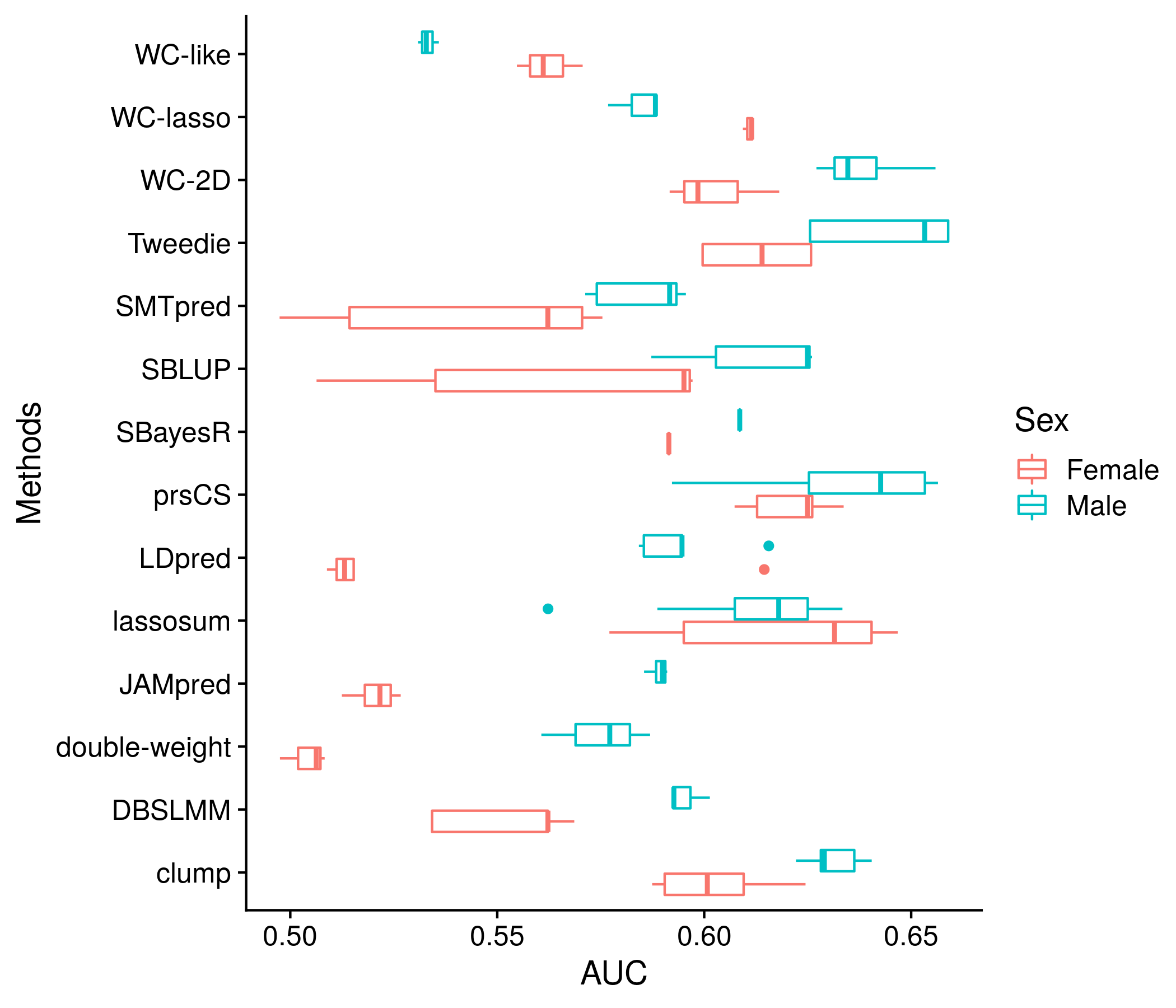
Figure 11.10: Example plot of the performance of each method (for all scores) by sex
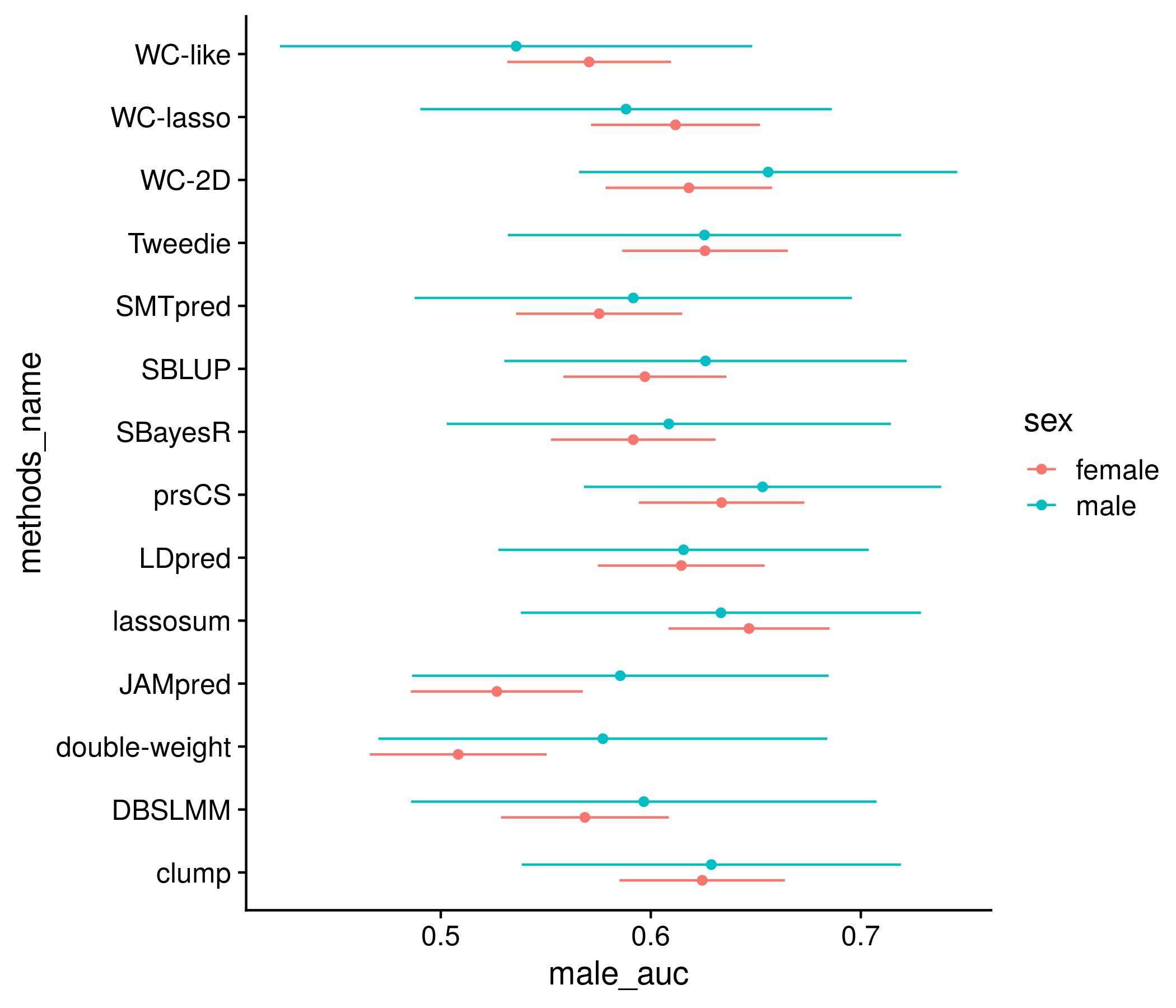
Figure 11.11: Example plot of the performance of each method (for the best score) by sex
The next section: comparison of ethnic groups. By default this comparison is only looking at the best score for each method. I found trying to depict each of the quantiles to be unwieldy and instead look at just the mean and SD of each score in each racial group. The only plot I make is that exact information through a series of dots and error bars.
#################################################################
##################### ETHNICITY ###############################
#################################################################


ethnic_res <- nonpred_res[["new_ethnic"]]
all_dist <- list()
all_param <- list()
i <- 1
k <- 1
for(ethnic in c("brit_stats", "euro_stats", "african_stats", "asian_stats")){
  for(j in 1:nrow(ethnic_res[[ethnic]])){
    all_dist[[i]] <- data.frame(score = rnorm(1000, mean = ethnic_res[[ethnic]][j,1], sd = ethnic_res[[ethnic]][j,2]))
    all_dist[[i]]$ethnic <- ethnic
    all_dist[[i]]$name <- ethnic_res[["names_to_keep"]][j]

    i <- i + 1
  }
  all_param[[k]] <- data.frame(ethnic_res[[ethnic]][,1:2])
  colnames(all_param[[k]]) <- c("mean", "sd")
  all_param[[k]]$ethnic <- ethnic
  all_param[[k]]$name <- ethnic_res[["names_to_keep"]][1:nrow(all_param[[k]])]
  k <- k + 1
}

all_dist <- do.call("rbind", all_dist) #can create normal distribution looking things from here
all_param <- do.call("rbind", all_param)
all_param$method <- convert_names(str_split(all_param$name, fixed("."), simplify = T)[,3])
for_convert <- cbind(c("brit_stats", "euro_stats", "african_stats", "asian_stats"), c("British", "European", "African", "Asian"))
all_param$ethnic <- convert_names(all_param$ethnic, for_convert)
all_param$method <- factor(all_param$method, levels =
                             all_param$method[all_param$ethnic == "African"][order(all_param$mean[all_param$ethnic == "African"])])

the_plot <- ggplot(all_param, aes(method, mean, color = ethnic)) + geom_point(position=position_dodge(width = 0.9)) + coord_flip() +
  geom_errorbar(position=position_dodge(width = 0.9), aes(ymin = mean-sd, ymax = mean+sd), width = 0.2) +
  labs(y = "Score", x = "Method", color = "Ethnicity") +
  geom_vline(xintercept = 1:length(unique(all_param$method)) + 0.5, color = "grey80")
plot(the_plot)
ggsave(paste0("meta_plots/", tolower(author), ".nonpred.ethnic.1.png"),
       the_plot, "png", height=6, width=7)
saveRDS(all_param, paste0("nonpred_results/derived_from_per_score/", author, ".ethnic.plot.RDS"))


ethnic_stat <- ethnic_res[["stat_test"]]
keep1 <- ethnic_stat$comp1
keep2 <- ethnic_stat$comp2
colnames(ethnic_stat) <- c(ethnic_res[["names_to_keep"]][-length(ethnic_res[["names_to_keep"]])], "eth1", "eth2")
saveRDS(ethnic_stat, paste0("nonpred_results/derived_from_per_score/", author, ".ethnic.tstat.RDS"))

ethnic_stat <- as.data.frame(ethnic_res[["pval_test"]])
ethnic_stat$comp1 <- keep1
ethnic_stat$comp2 <- keep2
colnames(ethnic_stat) <- c(ethnic_res[["names_to_keep"]][-length(ethnic_res[["names_to_keep"]])], "eth1", "eth2")
saveRDS(ethnic_stat, paste0("nonpred_results/derived_from_per_score/", author, ".ethnic.pval.RDS"))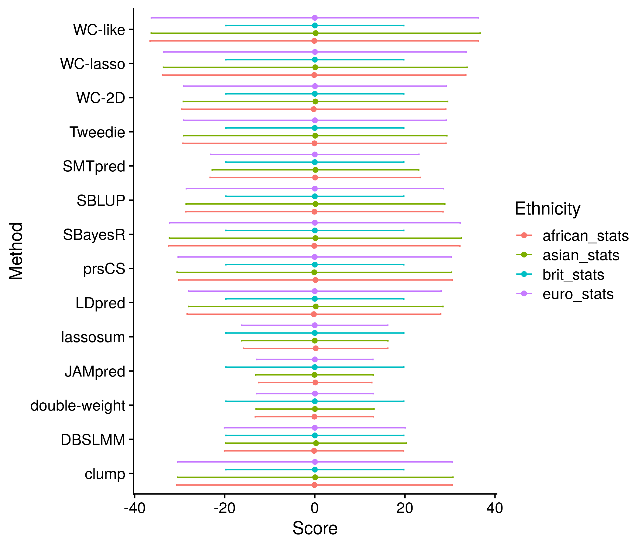
Figure 11.12: Example plot of the best scores’ mean and standard deviation for each method stratified by the ethnicities
The next section: sibling comparison. While it would be easy to follow the pattern of previous plots and depict all statistics together in a boxplot for each method, and a single best statistic for each method (the statistic here is concordance), I do not know how to say for sure what is the best in this case. Would best be based on sibling, non-sibling, both? Seeing as the method should be able to not favor one sibling group over all parameters I hope to be safe in only picking showing the box plot in this situation.
#################################################################
##################### SIBLING ###############################
#################################################################

sibs_res <- as.data.frame(nonpred_res[["sibs"]][[1]])

sibs_res$method <- convert_names(str_split(rownames(sibs_res), fixed("."), simplify = T)[,3])

sibs_res_sib <- sibs_res[,c(1:3,7)]
colnames(sibs_res_sib) <- c("lo", "conc", "hi", "method")
sibs_res_sib$type <- "Sibling"

sibs_res_non <- sibs_res[,c(4:7)]
colnames(sibs_res_non) <- c("lo", "conc", "hi", "method")
sibs_res_non$type <- "Non-Sib"

sibs_res <- rbind(sibs_res_sib, sibs_res_non)
mean_vals <- unlist(lapply(unique(sibs_res$method), function(x) mean(sibs_res$conc[sibs_res$method == x])))
sibs_res$method <- factor(sibs_res$method, levels = unique(sibs_res$method)[order(mean_vals)])

the_plot <- ggplot(sibs_res, aes(conc, method, color = type)) + geom_boxplot() +
  labs(x = "Concordance", y = "Method", color = "Comparison") +
  geom_hline(yintercept = 1:length(unique(sibs_res$method)) + 0.5, color = "grey80")
plot(the_plot)

ggsave(paste0("meta_plots/", tolower(author), ".nonpred.sibs.1.png"),
       the_plot, "png", height=6, width=7)
saveRDS(sibs_res, paste0("nonpred_results/derived_from_per_score/", author, ".sibs_res.plot.RDS"))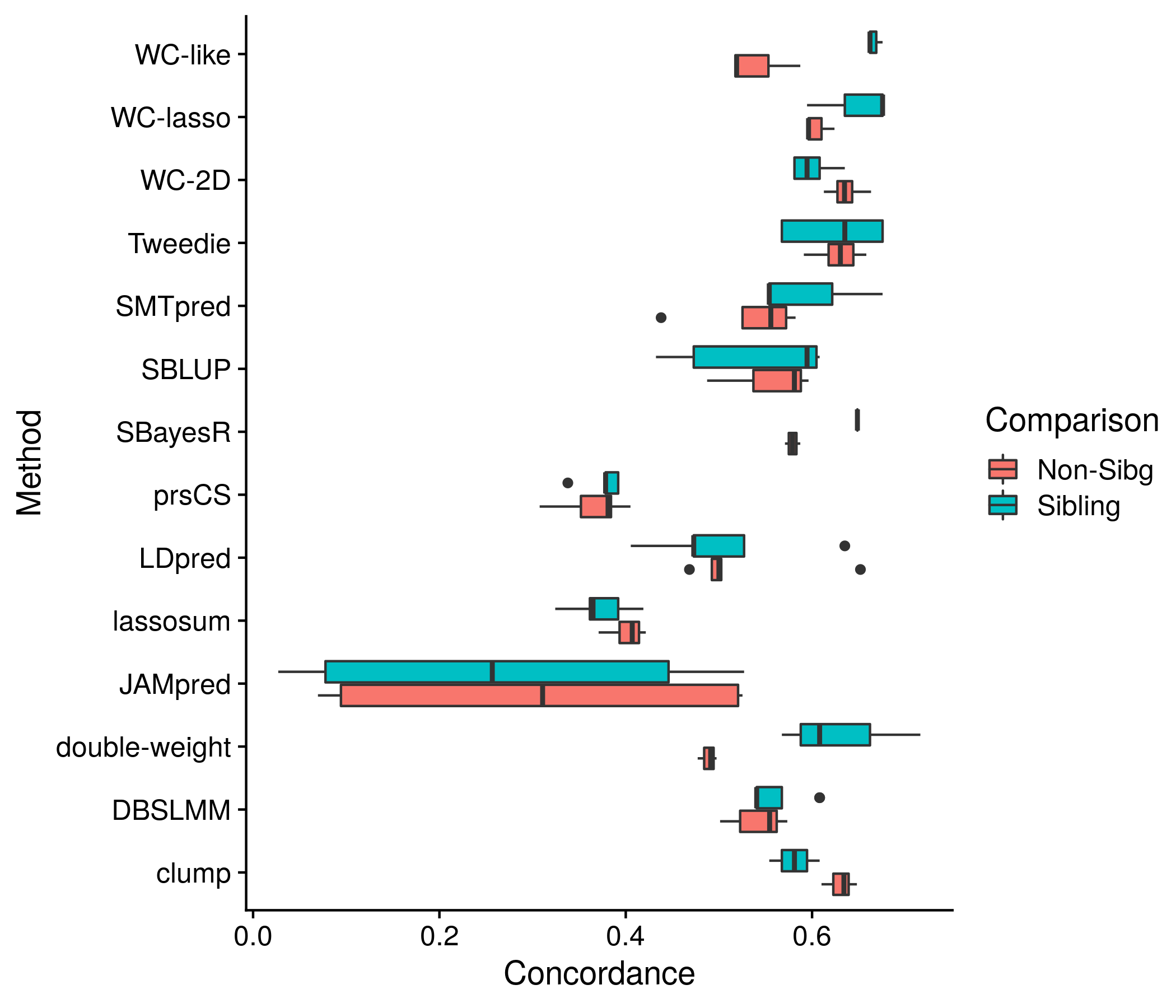
Figure 11.13: Example plot of the concordance for both sibling and non-sibling pairs for the best score for each method
The next section: age difference. The data being depicted here is very similar to the sex difference analysis. Therefore, the code and the plots themselves are very similar, and do not require much expounding.
#################################################################
##################### AGE DIFF ###############################
#################################################################


  age_res <- as.data.frame(nonpred_res[["age_diff"]])

  colnames(age_res) <- c("young_lo", "young_auc", "young_hi", "old_lo", "old_auc", "old_hi")
  age_res$score_name <- neat_score_names
  age_res$methods_name <- neat_method_names
  temp_save <- data.frame(age_res)

  plot_df <- melt(age_res, id.vars = c("score_name", "methods_name"))
  plot_df <- plot_df[plot_df$variable %in% c("young_auc", "old_auc"),]

  mean_vals <- unlist(lapply(unique(plot_df$methods_name), function(x) mean(plot_df$value[plot_df$methods_name == x])))
  plot_df$methods_name <- factor(plot_df$methods_name, levels = unique(plot_df$methods_name)[order(mean_vals)])
  the_plot <- ggplot(plot_df, aes(value, methods_name, color = variable)) + geom_boxplot() +
    labs(x = "AUC", y = "Methods", color = "Age\nGroup") +
    scale_color_discrete(labels = c("Young", "Old")) +
    geom_hline(yintercept = 1:length(unique(plot_df$methods_name)) + 0.5, color = "grey80")
  plot(the_plot)
  ggsave(paste0("meta_plots/", tolower(author), ".nonpred.agediff.1.png"),
         the_plot, "png", height=6, width=7)


  plot_df <- temp_save
  plot_df <- age_res[,c(1:3,7,8)]
  colnames(plot_df) <- c("old_lo", "old_auc", "old_hi", "score_name", "methods_name")
  plot_df <- rbind(plot_df, temp_save[,4:8])
  plot_df$sex <- c(rep("young", nrow(age_res)), rep("old", nrow(age_res)))

  plot_df <- plot_df[score_names %in% best_in_method[,1],]
  plot_df$sex <- str_to_title(plot_df$sex)
  plot_df$methods_name <- factor(plot_df$methods_name, levels =
                                   plot_df$methods_name[plot_df$sex == "Old"][order(plot_df$old_auc[plot_df$sex == "Old"])])
  the_plot <- ggplot(plot_df, aes(old_auc, methods_name, color = sex)) +
    geom_point(position = position_jitterdodge(jitter.width = 0, dodge.width = 0.5)) +
    geom_errorbarh(position = position_jitterdodge(jitter.width = 0, dodge.width = 0.5),
                   aes(xmin = old_lo, xmax = old_hi, height = 0)) +
    geom_hline(yintercept = 1:length(unique(plot_df$methods_name)) + 0.5, color = "grey80") +
    labs(x = "AUC", color = "Age\nGroup", y = "Methods")
  plot(the_plot)
  ggsave(paste0("meta_plots/", tolower(author), ".nonpred.agediff.2.png"),
         the_plot, "png", height=6, width=7)
  saveRDS(plot_df, paste0("nonpred_results/derived_from_per_score/", author, ".agediff.auc.RDS"))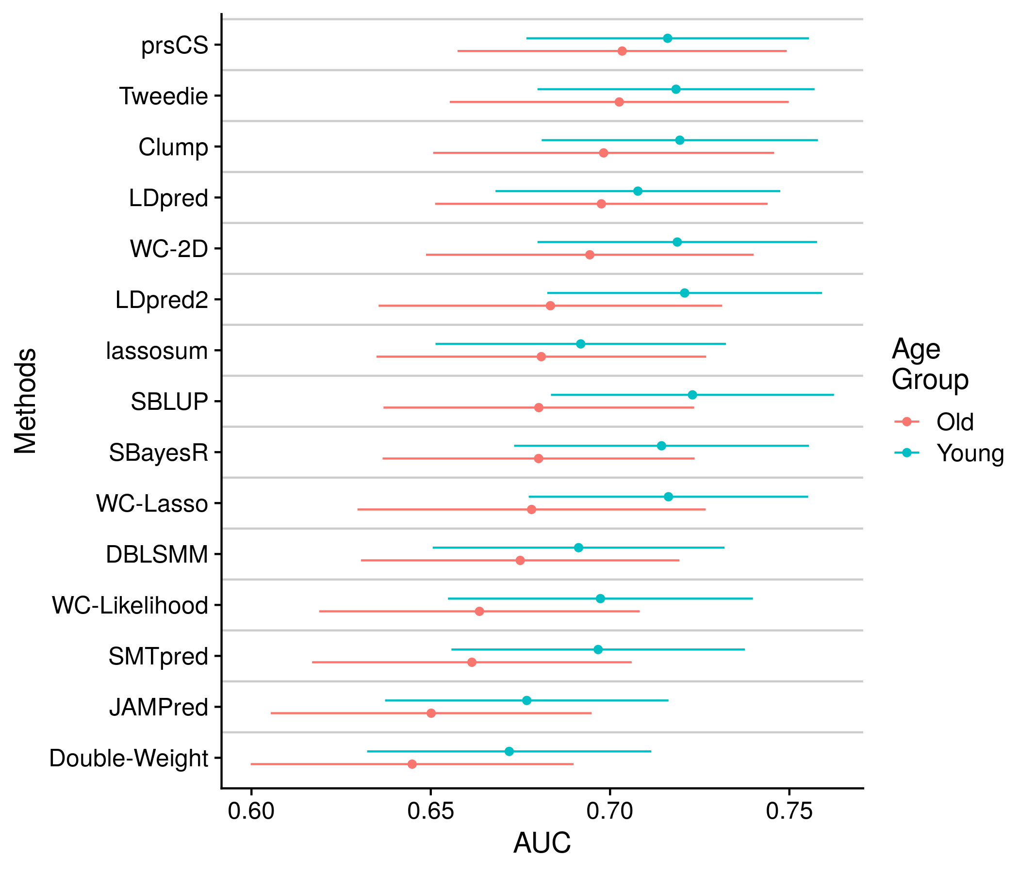
Figure 11.14: Example plot of the AUCs split by Age
The final section: many other personal attributed. Once again the plots and data are very similar, they are shown below for completness.
 #################################################################
  ##################### MANY OTHER AUC ###############################
  #################################################################


  vars_examined <- c("Time at\nCurrent\nAddress", "Income", "Number in\nHouse", "Year of\nEducation",
                     "Census:\nMedian Age", "Census:\nUnemployment", "Census:\nHealth", "Census:\nPop. Den.")
  var_splits <- list(c("1-20 years", "20+ years"), c("< 40,000", "> 40,000"), c("1-2 person", "3+ persons"),
                     c("1-19 years", "20+ years"), c("> 42 years", "< 42 years"), c("> 38", "< 38"),
                     c("> 719", "< 719"), c("> 32 persons/hectare", "< 32 persons/hectare"))
  all_plot_df <- list()
  all_pval_df <- list()

  for(var_ind in 1:length(vars_examined)){

    new_res <- as.data.frame(nonpred_res[["many_auc"]][[var_ind]])
    new_pval <- as.data.frame(nonpred_res[["many_pval"]][[var_ind]])

    colnames(new_res) <- c("bottom_lo", "bottom_auc", "bottom_hi", "upper_lo", "upper_auc", "upper_hi")
    new_res$score_name <- neat_score_names
    new_res$methods_name <- neat_method_names
    temp_save <- data.frame(new_res)

    plot_df <- melt(new_res, id.vars = c("score_name", "methods_name"))
    plot_df <- plot_df[plot_df$variable %in% c("bottom_auc", "upper_auc"),]

    mean_vals <- unlist(lapply(unique(plot_df$methods_name), function(x) mean(plot_df$value[plot_df$methods_name == x])))
    plot_df$methods_name <- factor(plot_df$methods_name, levels = unique(plot_df$methods_name)[order(mean_vals)])
    the_plot <- ggplot(plot_df, aes(value, methods_name, color = variable)) + geom_boxplot() +
      labs(x = "AUC", y = "Methods", color = vars_examined[var_ind]) +
      scale_color_discrete(labels = var_splits[[var_ind]]) +
      geom_hline(yintercept = 1:length(unique(plot_df$methods_name)) + 0.5, color = "grey80")
    plot(the_plot)
    ggsave(paste0("meta_plots/", tolower(author), ".nonpred.many.", var_ind, ".1.png"),
           the_plot, "png", height=6, width=7)


    plot_df <- temp_save
    plot_df <- new_res[,c(1:3,7,8)]
    colnames(plot_df) <- c("upper_lo", "upper_auc", "upper_hi", "score_name", "methods_name")
    plot_df <- rbind(plot_df, temp_save[,4:8])
    plot_df$var <- c(rep("young", nrow(new_res)), rep("old", nrow(new_res)))

    plot_df <- plot_df[score_names %in% best_in_method[,1],]

    plot_df$methods_name <- factor(plot_df$methods_name, levels =
                                     plot_df$methods_name[plot_df$var == "old"][order(plot_df$upper_auc[plot_df$var == "old"])])

    the_plot <- ggplot(plot_df, aes(upper_auc, methods_name, color = var)) +
      geom_point(position = position_jitterdodge(jitter.width = 0, dodge.width = 0.5)) +
      geom_errorbarh(position = position_jitterdodge(jitter.width = 0, dodge.width = 0.5),
                     aes(xmin = upper_lo, xmax = upper_hi, height = 0)) +
      geom_hline(yintercept = 1:length(unique(plot_df$methods_name)) + 0.5, color = "grey80") +
      labs(x = "AUC", color = vars_examined[var_ind], y = "Methods") +
      scale_color_discrete(labels = rev(var_splits[[var_ind]]))
    plot(the_plot)

    ggsave(paste0("meta_plots/", tolower(author), ".nonpred.many.", var_ind, ".2.png"),
           the_plot, "png", height=6, width=7)

    new_pval <- new_pval[score_names %in% best_in_method[,1],]
    plot_df$pval <- new_pval
    all_plot_df[[var_ind]] <- plot_df

    #new_pval$score_name <- neat_score_names
    #new_pval$methods_name <- neat_method_names
    #new_pval <- new_pval[score_names %in% best_in_method[,1],]
    #all_pval_df[[var_ind]] <- new_pval

  }

  saveRDS(all_plot_df, paste0("nonpred_results/derived_from_per_score/", author, ".many.auc.RDS"))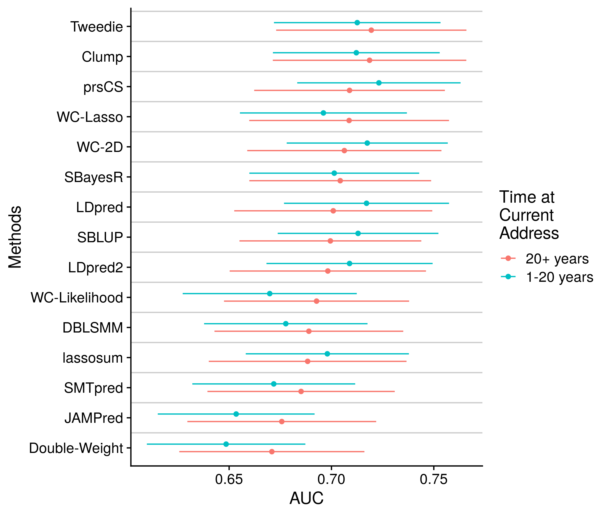
Figure 11.15: Example plot of the many other personal attributes examined wherein the attribute was used to split the sample and models were fit and assessed on each half